FM

Factorization Machines (FMs) are a supervised learning approach that enhances the linear regression model by incorporating the second-order feature interactions. Factorization Machine type algorithms are a combination of linear regression and matrix factorization, the cool idea behind this type of algorithm is it aims model interactions between features (a.k.a attributes, explanatory variables) using factorized parameters. By doing so it has the ability to estimate all interactions between features even with extremely sparse data.

Factorization machines (FM) [Rendle, 2010], proposed by Steffen Rendle in 2010, is a supervised algorithm that can be used for classification, regression, and ranking tasks. It quickly took notice and became a popular and impactful method for making predictions and recommendations. Particularly, it is a generalization of the linear regression model and the matrix factorization model. Moreover, it is reminiscent of support vector machines with a polynomial kernel. The strengths of factorization machines over the linear regression and matrix factorization are: (1) it can model χ -way variable interactions, where χ is the number of polynomial order and is usually set to two. (2) A fast optimization algorithm associated with factorization machines can reduce the polynomial computation time to linear complexity, making it extremely efficient especially for high dimensional sparse inputs. For these reasons, factorization machines are widely employed in modern advertisement and products recommendations.

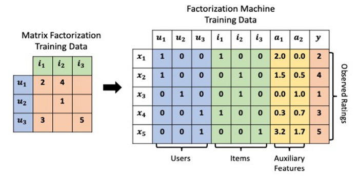
Most recommendation problems assume that we have a consumption/rating dataset formed by a collection of (user, item, rating) tuples. This is the starting point for most variations of Collaborative Filtering algorithms and they have proven to yield nice results; however, in many applications, we have plenty of item metadata (tags, categories, genres) that can be used to make better predictions. This is one of the benefits of using Factorization Machines with feature-rich datasets, for which there is a natural way in which extra features can be included in the model and higher-order interactions can be modeled using the dimensionality parameter d. For sparse datasets, a second-order FM model suffices, since there is not enough information to estimate more complex interactions.

$$f(x) = w_0 + \sum_{p=1}^Pw_px_p + \sum_{p=1}^{P-1}\sum_{q=p+1}^Pw_{p,q}x_px_q$$

This model formulation may look familiar — it's simply a quadratic linear regression. However, unlike polynomial linear models which estimate each interaction term separately, FMs instead use factorized interaction parameters: feature interaction weights are represented as the inner product of the two features' latent factor space embeddings:

$$f(x) = w_0 + \sum_{p=1}^Pw_px_p + \sum_{p=1}^{P-1}\sum_{q=p+1}^P\langle v_p,v_q \rangle x_px_q$$

This greatly decreases the number of parameters to estimate while at the same time facilitating more accurate estimation by breaking the strict independence criteria between interaction terms. Consider a realistic recommendation data set with 1,000,000 users and 10,000 items. A quadratic linear model would need to estimate U + I + UI ~ 10 billion parameters. A FM model of dimension F=10 would need only U + I + F(U + I) ~ 11 million parameters. Additionally, many common MF algorithms (including SVD++, ALS) can be re-formulated as special cases of the more general/flexible FM model class.

The above equation can be rewritten as:

$$\begin{align*} \hat{y}(\textbf{x}) = w_{0} + \sum_{i=1}^{n} w_{i} x_{i} + \sum_{i=1}^n \sum_{j=i+1}^n \hat{w}_{ij} x_{i} x_{j} \end{align*}$$

where,

• $w_0$ is the global bias
• $w_i$ denotes the weight of the i-th feature,
• $\hat{w}_{ij} = v_i^Tv_j$ denotes the weight of the cross feature $x_ix_j$
• $v_i \in \mathcal{R}^k$ denotes the embedding vector for feature $i$
• $k$ denotes the size of embedding vector

warning

For large, sparse datasets...FM and FFM is good. But for small, dense datasets...try to avoid.

Factorization machines appeared to be the method which answered the challenge!

	Accuracy	Speed	Sparsity
Collaborative Filtering	Too Accurate	Suitable	Suitable
SVM	Too Accurate	Suitable	Unsuitable
Random Forest/CART	General Accuracy	Unsuitable	Unsuitable
Factorization Machines (FM)	General Accuracy	Quick	Designed for it

To learn the FM model, we can use the MSE loss for regression task, the cross entropy loss for classification tasks, and the BPR loss for ranking task. Standard optimizers such as SGD and Adam are viable for optimization.

Despite effectiveness, FM can be hindered by its modelling of all feature interactions with the same weight, as not all feature interactions are equally useful and predictive. For example, the interactions with useless features may even introduce noises and adversely degrade the performance.

	For each	Learn
Linear	feature	a weight
Poly	feature pair	a weight
FM	feature	a latent vector
FFM	feature	multiple latent vectors

Adapt FM to implicit feedback

It’s not immediately obvious how to adapt FM models for implicit feedback data. One naïve approach would be to label all observed user-item interactions as $1$ and all unobserved interactions as $-1$ and train the model using a common classification loss function such as hinge or log loss. But with real-world recommendation data sets this would require the creation of billions of unobserved user-item training samples and result in a severe class imbalance due to interaction sparsity. This approach also has the same conceptual problem as the implicit feedback MF adaptation discussed above: it’s still minimizing rating prediction error instead of directly optimizing item rank-order.

Optimization techniques that learn rank-order directly instead of minimizing prediction error are referred to as Learning-to-Rank (LTR). LTR models train on pairs or lists of training samples instead of individual observations. The loss functions are based on the relative ordering of items instead of their raw scores. Models using LTR have produced state-of-the-art results in search, information retrieval, and collaborative filtering. These techniques are the key to adapting FM models to implicit feedback recommendation problems.

An Efficient Optimization Criterion

Optimizing the factorization machines in a straightforward method leads to a complexity of $\mathcal{O}(kd^2)$ as all pairwise interactions require to be computed. To solve this inefficiency problem, we can reorganize the third term of FM which could greatly reduce the computation cost, leading to a linear time complexity $\mathcal{O}(kd)$. The reformulation of the pairwise interaction term is as follows:

$$\begin{split}\begin{aligned} &\sum_{i=1}^d \sum_{j=i+1}^d \langle\mathbf{v}_i, \mathbf{v}_j\rangle x_i x_j \\ &= \frac{1}{2} \sum_{i=1}^d \sum_{j=1}^d\langle\mathbf{v}_i, \mathbf{v}_j\rangle x_i x_j - \frac{1}{2}\sum_{i=1}^d \langle\mathbf{v}_i, \mathbf{v}_i\rangle x_i x_i \\ &= \frac{1}{2} \big (\sum_{i=1}^d \sum_{j=1}^d \sum_{l=1}^k\mathbf{v}_{i, l} \mathbf{v}_{j, l} x_i x_j - \sum_{i=1}^d \sum_{l=1}^k \mathbf{v}_{i, l} \mathbf{v}_{i, l} x_i x_i \big)\\ &= \frac{1}{2} \sum_{l=1}^k \big ((\sum_{i=1}^d \mathbf{v}_{i, l} x_i) (\sum_{j=1}^d \mathbf{v}_{j, l}x_j) - \sum_{i=1}^d \mathbf{v}_{i, l}^2 x_i^2 \big ) \\ &= \frac{1}{2} \sum_{l=1}^k \big ((\sum_{i=1}^d \mathbf{v}_{i, l} x_i)^2 - \sum_{i=1}^d \mathbf{v}_{i, l}^2 x_i^2) \end{aligned}\end{split}$$

With this reformulation, the model complexity are decreased greatly. Moreover, for sparse features, only non-zero elements needs to be computed so that the overall complexity is linear to the number of non-zero features.

Links

1. http://d2l.ai/chapter_recommender-systems/fm.html