
· 2 min read
Sparsh Agarwal

Health insurance can be complicated—especially when it comes to prior authorization (also referred to as pre-approval, pre-authorization, and pre-certification). The manual labor involved in obtaining prior authorizations (PAs) is a well-recognized burden among providers. Up to 46% of PA requests are still submitted by fax, and 60% require a telephone call, according to America’s Health Insurance Plans (AHIP). A 2018 survey by the American Medical Association (AMA) found that doctors and their staff spend an average of 2 days a week completing PAs. In addition to eating up time that physicians could spend with patients, PAs also contribute to burnout.

The objective was to identify the patterns from data to create clinical decision making in Pre-Auth and improve the accuracy in a clinical decision based on historical data analysis.

Two use cases were identified. Use Case 1 - Supervised Learning Model - to aid clinicians in UM decision making. Tasks - Ingest Pre-authorization data from Mongo DB into the analytical environment, Exploratory Data Analysis and Feature Engineering, Train supervised analytical models, model validation and model selection, Create a web service to be plugged into the case processing flow to call the model, and Display the recommendation from the model on UI on the authorization review screen. Use Case 2 - Unsupervised Learning Model - to generate insights from the pre-authorization data. Tasks - Ingest Pre-authorization data from Mongo DB into the analytical environment, Cluster analysis, univariate and multivariate analysis, and Generate insights and display insights on the dashboard.

Final Deliverables - Model re-training (batch mode), validation and deployment code (python scripts) with Unix command line support, Documentation - PPT, Recorded video, Technical document, Flask API backend system, HTML/PHP Web App frontend UI integration, and Plotly Dash Supervised/Unsupervised learning and insights generation dashboard.

· 7 min read
Sparsh Agarwal

/img/content-blog-raw-blog-detectron-2-untitled.png

Introduction

Detectron 2 is a next-generation open-source object detection system from Facebook AI Research. With the repo you can use and train the various state-of-the-art models for detection tasks such as bounding-box detection, instance and semantic segmentation, and person keypoint detection.

The following is the directory tree of detectron 2:

detectron2
├─checkpoint <- checkpointer and model catalog handlers
├─config <- default configs and handlers
├─data <- dataset handlers and data loaders
├─engine <- predictor and trainer engines
├─evaluation <- evaluator for each dataset
├─export <- converter of detectron2 models to caffe2 (ONNX)
├─layers <- custom layers e.g. deformable conv.
├─model_zoo <- pre-trained model links and handler
├─modeling
│ ├─meta_arch <- meta architecture e.g. R-CNN, RetinaNet
│ ├─backbone <- backbone network e.g. ResNet, FPN
│ ├─proposal_generator <- region proposal network
│ └─roi_heads <- head networks for pooled ROIs e.g. box, mask heads
├─solver <- optimizer and scheduler builders
├─structures <- structure classes e.g. Boxes, Instances, etc
└─utils <- utility modules e.g. visualizer, logger, etc

Installation

%%time
!pip install -U torch==1.4+cu100 torchvision==0.5+cu100 -f https://download.pytorch.org/whl/torch_stable.html;
!pip install cython pyyaml==5.1;
!pip install -U 'git+https://github.com/cocodataset/cocoapi.git#subdirectory=PythonAPI';
!pip install detectron2 -f https://dl.fbaipublicfiles.com/detectron2/wheels/cu100/index.html;

from detectron2 import model_zoo
from detectron2.engine import DefaultPredictor
from detectron2.config import get_cfg
from detectron2.utils.visualizer import Visualizer
from detectron2.data import MetadataCatalog

Inference on pre-trained models

Original image

Original image

Object detection with Faster-RCNN-101

Object detection with Faster-RCNN-101

Instance segmentation with Mask-RCNN-50

Instance segmentation with Mask-RCNN-50

Keypoint estimation with Keypoint-RCNN-50

Keypoint estimation with Keypoint-RCNN-50

Panoptic segmentation with Panoptic-FPN-101

Panoptic segmentation with Panoptic-FPN-101

Default Mask R-CNN (top) vs. Mask R-CNN with PointRend (bottom) comparison

Default Mask R-CNN (top) vs. Mask R-CNN with PointRend (bottom) comparison

Fine-tuning Balloons Dataset

Load the data

# download, decompress the data
!wget https://github.com/matterport/Mask_RCNN/releases/download/v2.1/balloon_dataset.zip
!unzip balloon_dataset.zip > /dev/null

Convert dataset into Detectron2's standard format

from detectron2.structures import BoxMode
# write a function that loads the dataset into detectron2's standard format
def get_balloon_dicts(img_dir):
json_file = os.path.join(img_dir, "via_region_data.json")
with open(json_file) as f:
imgs_anns = json.load(f)

dataset_dicts = []
for _, v in imgs_anns.items():
record = {}

filename = os.path.join(img_dir, v["filename"])
height, width = cv2.imread(filename).shape[:2]

record["file_name"] = filename
record["height"] = height
record["width"] = width

annos = v["regions"]
objs = []
for _, anno in annos.items():
assert not anno["region_attributes"]
anno = anno["shape_attributes"]
px = anno["all_points_x"]
py = anno["all_points_y"]
poly = [(x + 0.5, y + 0.5) for x, y in zip(px, py)]
poly = list(itertools.chain.from_iterable(poly))

obj = {
"bbox": [np.min(px), np.min(py), np.max(px), np.max(py)],
"bbox_mode": BoxMode.XYXY_ABS,
"segmentation": [poly],
"category_id": 0,
"iscrowd": 0
}
objs.append(obj)
record["annotations"] = objs
dataset_dicts.append(record)
return dataset_dicts

from detectron2.data import DatasetCatalog, MetadataCatalog
for d in ["train", "val"]:
DatasetCatalog.register("balloon/" + d, lambda d=d: get_balloon_dicts("balloon/" + d))
MetadataCatalog.get("balloon/" + d).set(thing_classes=["balloon"])
balloon_metadata = MetadataCatalog.get("balloon/train")

Model configuration and training

from detectron2.engine import DefaultTrainer
from detectron2.config import get_cfg

cfg = get_cfg()
cfg.merge_from_file(model_zoo.get_config_file("COCO-InstanceSegmentation/mask_rcnn_R_50_FPN_3x.yaml"))
cfg.DATASETS.TRAIN = ("balloon/train",)
cfg.DATASETS.TEST = () # no metrics implemented for this dataset
cfg.DATALOADER.NUM_WORKERS = 2
cfg.MODEL.WEIGHTS = model_zoo.get_checkpoint_url("COCO-InstanceSegmentation/mask_rcnn_R_50_FPN_3x.yaml")
cfg.SOLVER.IMS_PER_BATCH = 2
cfg.SOLVER.BASE_LR = 0.00025
cfg.SOLVER.MAX_ITER = 300 # 300 iterations seems good enough, but you can certainly train longer
cfg.MODEL.ROI_HEADS.BATCH_SIZE_PER_IMAGE = 128 # faster, and good enough for this toy dataset
cfg.MODEL.ROI_HEADS.NUM_CLASSES = 1 # only has one class (ballon)

os.makedirs(cfg.OUTPUT_DIR, exist_ok=True)
trainer = DefaultTrainer(cfg)
trainer.resume_or_load(resume=False)
trainer.train()

Inference and Visualization

from detectron2.utils.visualizer import ColorMode

# load weights
cfg.MODEL.WEIGHTS = os.path.join(cfg.OUTPUT_DIR, "model_final.pth")
cfg.MODEL.ROI_HEADS.SCORE_THRESH_TEST = 0.7 # set the testing threshold for this model
# Set training data-set path
cfg.DATASETS.TEST = ("balloon/val", )
# Create predictor (model for inference)
predictor = DefaultPredictor(cfg)

dataset_dicts = get_balloon_dicts("balloon/val")
for d in random.sample(dataset_dicts, 3):
im = cv2.imread(d["file_name"])
outputs = predictor(im)
v = Visualizer(im[:, :, ::-1],
metadata=balloon_metadata,
scale=0.8,
instance_mode=ColorMode.IMAGE_BW # remove the colors of unsegmented pixels
)
v = v.draw_instance_predictions(outputs["instances"].to("cpu"))
cv2_imshow(v.get_image()[:, :, ::-1])

/img/content-blog-raw-blog-detectron-2-untitled-7.png

/img/content-blog-raw-blog-detectron-2-untitled-8.png

/img/content-blog-raw-blog-detectron-2-untitled-9.png

Fine-tuning Chip Dataset

Load the data

#get the dataset
!pip install -q kaggle
!pip install -q kaggle-cli
os.environ['KAGGLE_USERNAME'] = "sparshag"
os.environ['KAGGLE_KEY'] = "1b1f894d1fa6febe9676681b44ad807b"
!kaggle datasets download -d tannergi/microcontroller-detection
!unzip microcontroller-detection.zip

Convert dataset into Detectron2's standard format

# Registering the dataset
from detectron2.structures import BoxMode
def get_microcontroller_dicts(csv_file, img_dir):
df = pd.read_csv(csv_file)
df['filename'] = df['filename'].map(lambda x: img_dir+x)

classes = ['Raspberry_Pi_3', 'Arduino_Nano', 'ESP8266', 'Heltec_ESP32_Lora']

df['class_int'] = df['class'].map(lambda x: classes.index(x))

dataset_dicts = []
for filename in df['filename'].unique().tolist():
record = {}

height, width = cv2.imread(filename).shape[:2]

record["file_name"] = filename
record["height"] = height
record["width"] = width

objs = []
for index, row in df[(df['filename']==filename)].iterrows():
obj= {
'bbox': [row['xmin'], row['ymin'], row['xmax'], row['ymax']],
'bbox_mode': BoxMode.XYXY_ABS,
'category_id': row['class_int'],
"iscrowd": 0
}
objs.append(obj)
record["annotations"] = objs
dataset_dicts.append(record)
return dataset_dicts

classes = ['Raspberry_Pi_3', 'Arduino_Nano', 'ESP8266', 'Heltec_ESP32_Lora']
for d in ["train", "test"]:
DatasetCatalog.register('microcontroller/' + d, lambda d=d: get_microcontroller_dicts('Microcontroller Detection/' + d + '_labels.csv', 'Microcontroller Detection/' + d+'/'))
MetadataCatalog.get('microcontroller/' + d).set(thing_classes=classes)
microcontroller_metadata = MetadataCatalog.get('microcontroller/train')

Model configuration and training

# Train the model
cfg = get_cfg()
cfg.merge_from_file(model_zoo.get_config_file("COCO-Detection/faster_rcnn_R_101_FPN_3x.yaml"))
cfg.DATASETS.TRAIN = ('microcontroller/train',)
cfg.DATASETS.TEST = () # no metrics implemented for this dataset
cfg.DATALOADER.NUM_WORKERS = 2
cfg.MODEL.WEIGHTS = model_zoo.get_checkpoint_url("COCO-Detection/faster_rcnn_R_101_FPN_3x.yaml")
cfg.SOLVER.IMS_PER_BATCH = 2
cfg.SOLVER.MAX_ITER = 1000
cfg.MODEL.ROI_HEADS.NUM_CLASSES = 4

os.makedirs(cfg.OUTPUT_DIR, exist_ok=True)
trainer = DefaultTrainer(cfg)
trainer.resume_or_load(resume=False)
trainer.train()

/img/content-blog-raw-blog-detectron-2-untitled-10.png

/img/content-blog-raw-blog-detectron-2-untitled-11.png

Inference and Visualization

cfg.MODEL.WEIGHTS = os.path.join(cfg.OUTPUT_DIR, "model_final.pth")
cfg.MODEL.ROI_HEADS.SCORE_THRESH_TEST = 0.8 # set the testing threshold for this model
cfg.DATASETS.TEST = ('microcontroller/test', )
predictor = DefaultPredictor(cfg)

df_test = pd.read_csv('Microcontroller Detection/test_labels.csv')

dataset_dicts = DatasetCatalog.get('microcontroller/test')
for d in random.sample(dataset_dicts, 3):
im = cv2.imread(d["file_name"])
outputs = predictor(im)
v = Visualizer(im[:, :, ::-1],
metadata=microcontroller_metadata,
scale=0.8
)
v = v.draw_instance_predictions(outputs["instances"].to("cpu"))
cv2_imshow(v.get_image()[:, :, ::-1])

Real-time Webcam inference

from IPython.display import display, Javascript
from google.colab.output import eval_js
from base64 import b64decode

def take_photo(filename='photo.jpg', quality=0.8):
js = Javascript('''
async function takePhoto(quality) {
const div = document.createElement('div');
const capture = document.createElement('button');
capture.textContent = 'Capture';
div.appendChild(capture);

const video = document.createElement('video');
video.style.display = 'block';
const stream = await navigator.mediaDevices.getUserMedia({video: true});

document.body.appendChild(div);
div.appendChild(video);
video.srcObject = stream;
await video.play();

// Resize the output to fit the video element.
google.colab.output.setIframeHeight(document.documentElement.scrollHeight, true);

// Wait for Capture to be clicked.
await new Promise((resolve) => capture.onclick = resolve);

const canvas = document.createElement('canvas');
canvas.width = video.videoWidth;
canvas.height = video.videoHeight;
canvas.getContext('2d').drawImage(video, 0, 0);
stream.getVideoTracks()[0].stop();
div.remove();
return canvas.toDataURL('image/jpeg', quality);
}
''')
display(js)
data = eval_js('takePhoto({})'.format(quality))
binary = b64decode(data.split(',')[1])
with open(filename, 'wb') as f:
f.write(binary)
return filename

from IPython.display import Image
try:
filename = take_photo()
print('Saved to {}'.format(filename))

# Show the image which was just taken.
display(Image(filename))
except Exception as err:
# Errors will be thrown if the user does not have a webcam or if they do not
# grant the page permission to access it.
print(str(err))
model_path = '/content/output/model_final.pth'
config_path= model_zoo.get_config_file("COCO-Detection/faster_rcnn_R_101_FPN_3x.yaml")

# Create config
cfg = get_cfg()
cfg.merge_from_file(config_path)
cfg.MODEL.ROI_HEADS.SCORE_THRESH_TEST = 0.1
cfg.MODEL.WEIGHTS = model_path

predictor = DefaultPredictor(cfg)

im = cv2.imread('photo.jpg')
outputs = predictor(im)

v = Visualizer(im[:, :, ::-1], MetadataCatalog.get(cfg.DATASETS.TRAIN[0]), scale=1.2)
v = v.draw_instance_predictions(outputs["instances"].to("cpu"))
cv2_imshow(v.get_image()[:, :, ::-1])

Fine-tuning on Face dataset

The process is same. Here is the output.

/img/content-blog-raw-blog-detectron-2-untitled-12.png

/img/content-blog-raw-blog-detectron-2-untitled-13.png

/img/content-blog-raw-blog-detectron-2-untitled-14.png

Behind the scenes

/img/content-blog-raw-blog-detectron-2-untitled-15.png

References

· 6 min read
Sparsh Agarwal

The usage and importance of recommender systems are increasing at a fast pace. And deep learning is gaining traction as the preferred choice for model architecture. Giants like Google and Facebook are already using recommenders to earn billions of dollars.

Recently, Facebook shared its approach to maintain its 12 trillion parameter recommender. Building these large systems is challenging because it requires huge computation and memory resources. And we will soon enter into 100 trillion range. And SMEs will not be left behind due to open-source environment of software architectures and the decreasing cost of hardware, especially on the cloud infrastructure.

As per one estimate, a model with 100 trillion parameters would require at least 200TB just to store the model, even at 16-bit floating-point accuracy. So we need architectures that can support efficient and distributed training of recommendation models.

Memory-intensive vs Computation-intensive: The increasing parameter comes mostly from the embedding layer which maps each entrance of an ID type feature (such as an user ID and a session ID) into a fixed length low-dimensional embedding vector. Consider the billion scale of entrances for the ID type features in a production recommender system and the wide utilization of feature crosses, the embedding layer usually domains the parameter space, which makes this component extremely memory-intensive. On the other hand, these low-dimensional embedding vectors are concatenated with diversified Non-ID type features (e.g., image, audio, video, social network, etc.) to feed a group of increasingly sophisticated neural networks (e.g., convolution, LSTM, multi-head attention) for prediction(s). Furthermore, in practice, multiple objectives can also be combined and optimized simultaneously for multiple tasks. These mechanisms make the rest neural network increasingly computation-intensive.

An example of a recommender models with 100+ trillions of parameter in the embedding layer and 50+ TFLOP computation in the neural network.

An example of a recommender models with 100+ trillions of parameter in the embedding layer and 50+ TFLOP computation in the neural network.

Alibaba's XDL, Baidu's PaddleRec, and Kwai's Persia are some open-source frameworks for this large-scale distributed training of recommender systems.

Parameter Server Framework

Existing distributed systems for deep learning based recommender models are usually built on top of the parameter server (PS) framework, where one can add elastic distributed storage to hold the increasingly large amount of parameters of the embedding layer. On the other hand, the computation workload does not scale linearly with the increasing parameter scale of the embedding layer—in fact, with an efficient implementation, a lookup operation over a larger embedding table would introduce almost no additional computations.

Left: deep learning based recommender model training workflow over a heterogeneous cluster. Right: Gantt charts to compare fully synchronous, fully asynchronous, raw hybrid and optimized hybrid modes of distributed training of the deep learning recommender model. [Source](https://arxiv.org/pdf/2111.05897v1.pdf).

Left: deep learning based recommender model training workflow over a heterogeneous cluster. Right: Gantt charts to compare fully synchronous, fully asynchronous, raw hybrid and optimized hybrid modes of distributed training of the deep learning recommender model. Source.

PERSIA

PERSIA (Parallel rEcommendation tRaining System with hybrIAcceleration) is a PyTorch-based system for training deep learning recommendation models on commodity hardware. It supports models containing more than 100 trillion parameters.

It uses a hybrid training algorithm to tackle the embedding layer and dense neural network modules differently—the embedding layer is trained in an asynchronous fashion to improve the throughput of training samples, while the rest neural network is trained in a synchronous fashion to preserve the statistical efficiency.

It also uses a distributed system to manage the hybrid computation resources (CPUs and GPUs) to optimize the co-existence of asynchronicity and synchronicity in the training algorithm.

Untitled

Untitled

Persia includes a data loader module, a embedding PS (Parameter Server) module, a group of embedding workers over CPU nodes, and a group of NN workers over GPU instances. Each module can be dynamically scaled for different model scales and desired training throughput:

  • A data loader that fetches training data from distributed storages such as Hadoop, Kafka, etc;
  • A embedding parameter server (embedding PS for short) manages the storage and update of the parameters in the embedding layer $\mathrm{w}^{emb}$;
  • A group of embedding workers that runs Algorithm 1 for getting the embedding parameters from the embedding PS; aggregating embedding vectors (potentially) and putting embedding gradients back to embedding PS;
  • A group of NN workers that runs the forward-/backward- propagation of the neural network $\mathrm{NN_{w^{nn}}(·)}$.

The architecture of Persia.

The architecture of Persia.

Logically, the training procedure is conducted by Persia in a data dispatching based paradigm as below:

  1. The data loader will dispatch the ID type feature $\mathrm{x^{ID}}$ to an embedding worker—the embedding worker will generate an unique sample ID 𝜉 for this sample, buffer this sample ID with the ID type feature $\mathrm{x_\xi^{ID}}$ locally, and returns this ID 𝜉 back the data loader; the data loader will associate this sample’s Non-ID type features and labels with this unique ID.
  2. Next, the data loader will dispatch the Non-ID type feature and label(s) $\mathrm{(x\xi^{NID},y\xi)}$ to a NN worker.
  3. Once a NN worker receives this incomplete training sample, it will issue a request to pull the ID type features’ $\mathrm{(x\xi^{ID})}$ embedding $\mathrm{w\xi^{emb}}$ from some embedding worker according to the sample ID 𝜉—this would trigger the forward propagation in Algorithm 1, where the embedding worker will use the buffered ID type feature $\mathrm{x\xi^{ID}}$ to get the corresponding $\mathrm{w\xi^{emb}}$ from the embedding PS.
  4. Then the embedding worker performs some potential aggregation of original embedding vectors. When this computation finishes, the aggregated embedding vector $\mathrm{w_\xi^{emb}}$ will be transmitted to the NN worker that issues the pull request.
  5. Once the NN worker gets a group of complete inputs for the dense module, it will create a mini-batch and conduct the training computation of the NN according to Algorithm 2. Note that the parameter of the NN always locates in the device RAM of the NN worker, where the NN workers synchronize the gradients by the AllReduce Paradigm.
  6. When the iteration of Algorithm 2 is finished, the NN worker will send the gradients of the embedding ($\mathrm{F_\xi^{emb'}}$) back to the embedding worker (also along with the sample ID 𝜉).
  7. The embedding worker will query the buffered ID type feature $\mathrm{x\xi^{ID}}$ according to the sample ID 𝜉; compute gradients $\mathrm{F\xi^{emb'}}$ of the embedding parameters and send the gradients to the embedding PS, so that the embedding PS can finally compute the updates according the embedding parameter’s gradients by its SGD optimizer and update the embedding parameters.

· 2 min read
Sparsh Agarwal

/img/content-blog-raw-blog-document-recommendation-untitled.png

Introduction

Business objective

For the given user query, recommend relevant documents (BRM_ifam)

Technical objective

1-to-N mapping of given input text

Proposed Framework 1 — Hybrid Recommender System

  • Text → Vector (Universal Sentence Embedding with TF Hub)
  • Vector → Content-based Filtering Recommendation
  • Index → Interaction Matrix
  • Interaction Matrix → Collaborative Filtering Recommendation
  • Collaborative + Content-based → Hybrid Recommendation
  • Evaluation: Area-under-curve

Proposed Framework 2 — Content-based Recommender System

  1. Find A most similar user → Cosine similarity
  2. For each user in A, find TopK Most Similar Items → Map Argsort
  3. For each item Find TopL Most Similar Items → Cosine similarity
  4. Display
  5. Implement an evaluation metric
  6. Evaluate

Results and Discussion

  • build.py → this script will take the training data as input and save all the required files in the same working directory
  • recommend.py → this script will take the user query as input and predict top-K BRM recommendations

Variables (during recommendation, you will be asked 2–3 choices, the meaning of those choices are as following)

  • top-K — how many top items you want to get in recommendation
  • secondary items: this will determine how many similar items you would like to add in consideration, for each primary matching item
  • sorted by frequency: since multiple input queries might point to same output, therefore this option allows to take that frequence count of outputs in consideration and will move the more frequent items at the top.

Code

https://gist.github.com/sparsh-ai/4e5f06ba3c55192b33a276ee67dbd42c#file-text-recommendations-ipynb

· 3 min read
Sparsh Agarwal

/img/content-blog-raw-blog-fake-voice-detection-untitled.png

Introduction

Fake audio can be used for malicious purposes which affect directly or indirectly human life. The objective is to differentiate between fake and real voice. Python and deep learning has been used and implemented to achieve the objective. Audio files or video file are being used as an input of this work then model has been trained for uniquely identify features for voice creation and voice detection. Deep learning technique is used to find accuracy between real and fake.

Speaker recognition usually refers to both speaker identification and speaker verification. A speaker identification system identifies who the speaker is, while an automatic speaker verification (ASV) system decides if an identity claim is true or false. A general ASV system is robust to zero-effort impostors, they are vulnerable to more sophisticated attacks. Such vulnerability represents one of the security concerns of ASV systems. Spoofing involves an adversary (attacker) who masquerades as the target speaker to gain the access to a system. Such spoofing attacks can happen to various biometric traits, such as fingerprints, iris, face, and voice patterns. We are focusing only on the voice-based spoofing and anti-spoofing techniques for ASV system. The spoofed speech samples can be obtained through speech synthesis, voice conversion, or replay of recorded speech. Imagine the following scenario… Your phone rings, you pick up. It’s your spouse asking you for details about your savings account — they don’t have the account information on hand, but want to deposit money there this afternoon. Later, you realize a bunch of money has went missing! After investigating, you find out that the person masquerading as them on the other line was a voice 100% generated with AI. You’ve just been scammed, and on top of that, can’t believe the voice you thought belonged to your spouse was actually a fake.

To discern between real and fake audio, the detector uses visual representations of audio clips called spectrograms, which are also used to train speech synthesis models. Google’s 2019 AVSSpoof dataset contains over 25,000 clips of audio, featuring both real and fake clips of a variety of male and female speakers.Temporal Convolution Model

Modeling Approach

First, raw audio is preprocessed and converted into a mel-frequency spectrogram — this is the input for the model. The model performs convolutions over the time dimension of the spectrogram, then uses masked pooling to prevent overfitting. Finally, the output is passed into a dense layer and a sigmoid activation function, which ultimately outputs a predicted probability between 0 (fake) and 1 (real). The baseline model achieved 99%, 95%, and 85% accuracy on the train, validation, and test sets respectively. The differing performance is caused by differences between the three datasets. While all three datasets feature distinct and different speakers, the test set uses a different set of fake audio generating algorithms that were not present in the train or validation set.

Proposed Framework

Process Flow

  • Voice detection
    • Temporal Convolution model
      • Install packages
      • Download pretrained models
      • Initialize the model
      • Load data
      • Detect DeepFakes
    • GMM-UBG model
      • Install packages
      • Train the model
      • Load data
      • Detect DeepFakes
    • Convolutional VAE model
      • Install packages
      • Train the model
      • Load data
      • Detect DeepFakes
    • Voice Similarity
      • Install packages
      • Load data
      • Voice similarity match
      • Embedding visualization

Models Algorithms

  1. Temporal Convolution
  2. ResNet
  3. GMM
  4. Light CNN
  5. Fusion
  6. SincNet
  7. ASSERT
  8. HOSA
  9. CVAE

· 4 min read
Sparsh Agarwal

/img/content-blog-raw-blog-image-similarity-system-untitled.png

Choice of variables

Image Encoder

We can select any pre-trained image classification model. These models are commonly known as encoders because their job is to encode an image into a feature vector. I analyzed four encoders named 1) MobileNet, 2) EfficientNet, 3) ResNet and 4) BiT. After basic research, I decided to select BiT model because of its performance and state-of-the-art nature. I selected the BiT-M-50x3 variant of model which is of size 748 MB. More details about this architecture can be found on the official page here.

Vector Similarity System

Images are represented in a fixed-length feature vector format. For the given input vector, we need to find the TopK most similar vectors, keeping the memory efficiency and real-time retrival objective in mind. I explored the most popular techniques and listed down five of them: Annoy, Cosine distance, L1 distance, Locally Sensitive Hashing (LSH) and Image Deep Ranking. I selected Annoy because of its fast and efficient nature. More details about Annoy can be found on the official page here.

Dataset

I listed down 3 datasets from Kaggle that were best fitting the criteria of this use case: 1) Fashion Product Images (Small), 2) Food-11 image dataset and 3) Caltech 256 Image Dataset. I selected Fashion dataset and Foods dataset.

Literature review

  • Determining Image similarity with Quasi-Euclidean Metric arxiv
  • CatSIM: A Categorical Image Similarity Metric arxiv
  • Central Similarity Quantization for Efficient Image and Video Retrieval arxiv
  • Improved Deep Hashing with Soft Pairwise Similarity for Multi-label Image Retrieval arxiv
  • Model-based Behavioral Cloning with Future Image Similarity Learning arxiv
  • Why do These Match? Explaining the Behavior of Image Similarity Models arxiv
  • Learning Non-Metric Visual Similarity for Image Retrieval arxiv

Process Flow

Step 1: Data Acquisition

Download the raw image dataset into a directory. Categorize these images into their respective category directories. Make sure that images are of the same type, JPEG recommended. We will also process the metadata and store it in a serialized file, CSV recommended.

Step 2: Encoder Fine-tuning

Download the pre-trained image model and add two additional layers on top of that: the first layer is a feature vector layer and the second layer is the classification layer. We will only train these 2 layers on our data and after training, we will select the feature vector layer as the output of our fine-tuned encoder. After fine-tuning the model, we will save the feature extractor for later use.

Fig: a screenshot of encoder fine-tuning process

Fig: a screenshot of encoder fine-tuning process

Step 3: Image Vectorization

Now, we will use the encoder (prepared in step 2) to encode the images (prepared in step 1). We will save feature vector of each image as an array in a directory. After processing, we will save these embeddings for later use.

Step 4: Metadata and Indexing

We will assign a unique id to each image and create dictionaries to locate information of this image: 1) Image id to Image name dictionary, 2) Image id to image feature vector dictionary, and 3) (optional) Image id to metadata product id dictionary. We will also create an image id to image feature vector indexing. Then we will save these dictionaries and index object for later use.

Step 5: API Call

We will receive an image from user, encode it with our image encoder, find TopK similar vectors using Indexing object, and retrieve the image (and metadata) using dictionaries. We send these images (and metadata) back to the user.

Deployment

The API was deployed on AWS cloud infrastructure using AWS Elastic Beanstalk service.

/img/content-blog-raw-blog-image-similarity-system-untitled-2.png

· 10 min read
Sparsh Agarwal

Author: Alexsoft

In a hyper-connected world, where advanced analytics and smart devices constantly re-assess and monitor risks, the traditional once-a-year insurance policy looks increasingly irrelevant and static. Insurance will become a breathing and living thing that shrinks and scales with time to accommodate the changing risks in the clients’ daily lives. As technology continues to expand, real-time data from connected devices and predictive analysis from AIs and machine learning will enhance personalized insurance to benefit the client and insurer.

To satisfy the expectations of clients, insurers may need to go beyond the personalization of marketing communication and start personalizing product bundles for individuals.

What is personalized insurance?

Personalized insurance is the process of reaching insurance customers with targeted pricing, offers, and messages at the right time. Personalization spans across various types of insurance services, from health to property insurance.

Some insurers are already defining themselves as trusted advisors aiding people in navigating, anticipating, and eliminating risks rather than just paying the compensation when things go wrong.

For example, these companies use customer data from wearable and smart devices to monitor the user’s lifestyle. If the user’s data indicate the emergence of a serious medical condition, they can send the customer content designed to change their detrimental lifestyle or recommend immediate treatment. When the customer stays fit, healthy and does not carry out risky activities, their insurance cost will be decreased.

/img/content-blog-raw-blog-insurance-personalization-untitled.png

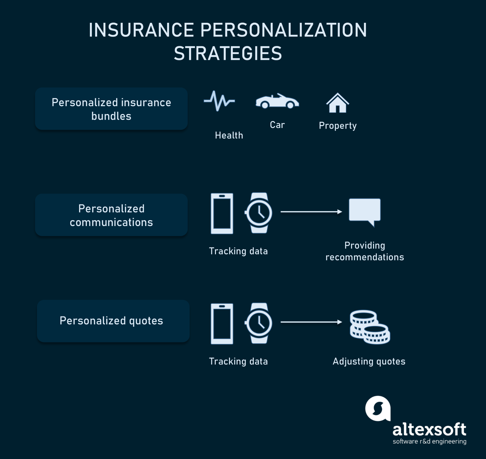
Insurers can provide personalization to customers at different levels:

  • Personalized product bundles. The insurer offers a wide range of products such as health, car, life, and property insurance. So, clients can choose the specific products they want and group them in a bundle.
  • Personalized communications. Insurers use data collected from smart devices to notify customers about harmful activities and lifestyles. They also send recommendations on lifestyle changes. Some insurers take a step further to provide clients with incentives for a healthy lifestyle.
  • Personalized insurance quote. Customers are able to adjust the price of their insurance premiums by turning off the ones they don’t need at any time. Some insurers enable automatic quote adjustments depending on customer’s behavior (e.g., driving habits) or lifestyle choices (e.g., exercising).

Why is it important?

Collecting and analyzing user data is vital in personalizing products based on individual behavior and preferences. In addition, insurers should use this data to enhance external relationships with their customers and guide their internal processes. This will eventually lead to delightful customer experiences and efficient operations.

Personalized insurance is important for many reasons:

Customers expect personalized treatment. Every customer wants to feel special, and the personalization of your services and products will do just that. It will make them stay loyal to you. Moreover, customers are open for personalization. According to the Accenture study, 95 percent of new customers are ready to share their data in exchange for personalized insurance services. And about 58 percent of conservative users would be willing to do so.

Driving more effective sales and increasing revenue. Personalization benefits your sales and income in two ways. First, lots of people are ready to share their data with you in exchange for incentives and reduced premiums. Secondly, having access to clients’ data gives you the ability to target people who are already interested in your product, thereby increasing sales and revenue at a lower cost. You will be able to reach your customers at the right time and with the product they need.

Streamlining operations and working with customers more accurately. Having an insight into customer preferences and behavior is crucial if you want to provide personalized services. Data obtained from social media activity, fitness trackers, GPS, and other tech can help you serve customers better.

Success stories

Lemonade

Use of AI and chatbots to personalize communications.

Lemonade is a US insurance company that uses Maya – an AI-powered bot, to collect and analyze customer data. Maya acts as a virtual assistant that gets information, provides quotes, and handles payments. It also has the ability to provide customized answers to user’s questions and even help them make changes to existing policies. Lemonade uses Natural Action Synthesis and Natural Language Processing to ensure that Maya gets smarter the more it chats. This is possible because their machine learning model is retrained almost daily.

/img/content-blog-raw-blog-insurance-personalization-untitled-1.png

On top of that, the company uses big data analytics to quantify losses and predict risks by placing the client into a risk group and quoting a relevant premium. Customers are grouped according to their risk behaviors. The groups are created using algorithms that collect extensive customer data, such as health conditions.
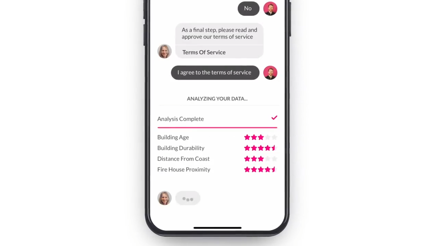
Cover

Cover is a US-based insurance metasearch company that notifies its clients of price drops for their premiums. Their technology works by scanning the market, looking for discounted and lowered prices of insurance premiums for their clients. Cover blends automation, mobile technology, and expert advice to provide customers with high-quality insurance protection at the best prices.

Cover compares with policy data and prices from over 30 different insurers. From the start, the customers need to provide answers to some questions, which will be used to match the client with a policy that suits their needs.

Oscar

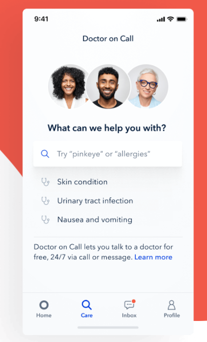
Oscar is a health insurer that provides its clients with a concierge team of medical professionals who give health advice and help them know if they see the best specialist for their specific health condition. They also help with finding the best doctors that accept Oscar insurance and manage and treat chronic conditions. Also, they set aside a separate concierge team in cases of emergencies that helps with the patient’s discharge and follow-up care.

Oscar’s mobile app acts as an intermediary between the user and the health system. The platform facilitates the customer’s interaction with their healthcare professionals. Clients can receive their lab reports, medical records, physician recommendations, and virtual care from the app. Oscar has also improved its high-touch services, including telemedicine and an “Ask your concierge” feature that connects users with a health insurance advice team.
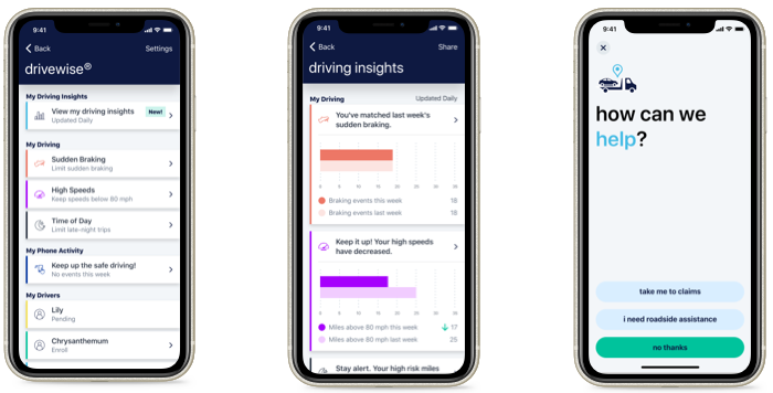
/img/content-blog-raw-blog-insurance-personalization-untitled-2.png

Alllstate

Allstate is an auto insurance company that offers personalized car insurance to its customers using telematics programs called Drivewise and Milewise. Drivewise is offered through a mobile app that monitors the customers driving behavior and provides feedback after each drive. Customers also receive incentives for safe driving. From the app interface, clients can check their rewards and driving behavior for the last 100 trips. The customer’s premium is then calculated based on factors like speeding, abrupt braking, and time of the trip. One of the nice things about Drivewise is that even those who do not have an Allstate care insurance policy can participate in this program. Their Milewise program, as the name suggests, lets customers pay insurance based on the miles covered. So, the app monitors the distance covered by the car, and low-mileage drivers can save on insurance.

/img/content-blog-raw-blog-insurance-personalization-untitled-3.png

How to approach personalization?

/img/content-blog-raw-blog-insurance-personalization-untitled-4.png

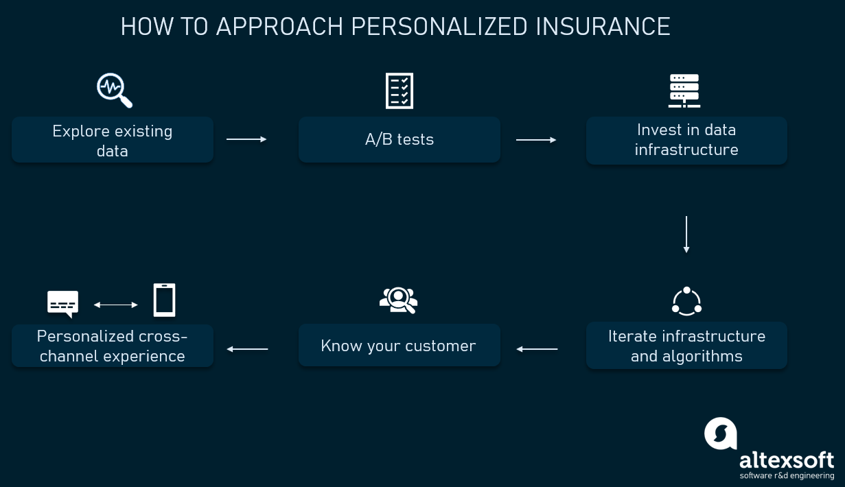
Before fully investing in personalization, you need to carefully plan your approach. This will ensure you have all the pieces for success, and it will help you follow through with your plan.

Explore existing data

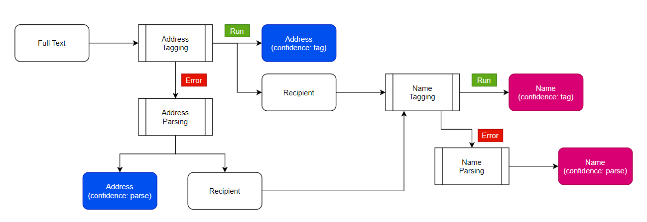
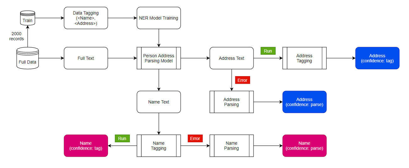
Having customer data is the minimum requirement to provide personalized services. First, you need to envision the type of personalization you want to offer. Then, make sure you have data collection channels that provide you with relevant data needed for your tasks. For instance, some of your documents may contain the required information, and you have to digitize, structure those, or extract specific details for that. So, you should audit your current information and data collection mechanisms to estimate whether you’ll need any additional effort to gather this data. For instance, you may want to use intelligent document processing.

Engage data scientists to make the proof of concept and carry out A/B tests

Your vision on personalization may not work for every business model. Or your data quality may be low to reach project feasibility. We’ve talked about that while explaining how to approach ROI calculations with machine learning projects. So, you need to present the data you have to a data science team to run several experiments and build prototypes. Once they are ready, you can roll out your new algorithms for a subset of customers to run A/B tests. Their results may show that the conventional approaches work better for you or help iterate on your assumptions.

Invest in data infrastructure

If the A/B tests show that personalization will work for your business model, that is where automation comes into play. You can start investing in data infrastructure and analytical pipelines to automate data collection and analysis mechanisms.

You’ll need a data engineering team for that. These specialists set up connections with data sources, such as mobile, IoT, and telematics devices, enable automatic data preparation, configure storages, and integrate your infrastructure with business intelligence software that helps explore and visualize data.

Continuously learn your customers’ preferences and needs

The data you collect is only as good as the insights gained from it. That is why it is vital to have a comprehensive analytic solution. A high-quality analytic software will transform the data into your most valuable asset. This data will be used to improve product development, make more accurate decisions, and provide personalized services to your customers.

Iterate on your infrastructure and algorithms

Personalization isn’t a one-time project. Whether you apply machine learning or build personalization based on rule-based systems, you still have to revisit your technology, continuously gather new data, and adapt your workflows.

Ensure a personalized cross-channel experience

Since the data collected from IoT devices and other tech is vital for personalization, it is important to make the customer experience seamless across different communication channels. Therefore, the customer should always be provided with the same level of personalization regardless of the touchpoint.

Challenges

Personalization is financially intensive. The ability of insurers to personalize insurance differs only marginally between marketing communications and products. Most of them, especially startups, do not have the funds to implement advanced technologies like machine learning needed for personalized insurance. However, insurers do not need to start with all the levels of personalization. They can often start by customizing their customer service, gathering data and insights, and then gradually developing towards more complex systems.

Complex process involving multiple parties. Also, it is difficult to balance personalization with financial targets, especially when establishing a price for risk. In-depth personalization of insurance must use data analytics from different sources to ensure that personalized offers reflect the client’s needs as well as the profitability and risks implications for the company.

Customer data is heavily regulated. Customer data from different sources are subject to industry regulations and privacy concerns. It is often a difficult task to obtain approval from regulators to use this data. Also, customers are becoming more aware of how companies are using their data and approve strict regulations. That is why laws such as General Data Protection Regulation (GDPR) and California Consumer Privacy Act (CCPA) have been passed, which gives customers more control over their data. Insurers can address this barrier by explaining to people how their systems work and how personal data is used. Read more on explainable machine learning in our dedicated article. Besides being open, insurers can provide clients with incentives and other services for free in exchange for access to personal data.

· 4 min read
Sparsh Agarwal

/img/content-blog-raw-blog-name-&amp;-address-parsing-untitled.png

Introduction

Create an API that can parse and classify names and addresses given a string. We tried probablepeople and usaddress. These work well separately but need the functionality of these packages combined, and better accuracy than what probablepeople provides. For the API, I'd like to mimic this with some minor modifications. A few examples:

  • "KING JOHN A 5643 ROUTH CREEK PKWY #1314 RICHARDSON TEXAS 750820146 UNITED STATES OF AMERICA" would return type: person; first_name: JOHN; last_name: KING; middle: A; street_address: 5643 ROUTH CREEK PKWY #1314; city: RICHARDSON; state: TEXAS; zip: 75082-0146; country: UNITED STATES OF AMERICA.
  • "THRM NGUYEN LIVING TRUST 2720 SUMMERTREE CARROLLTON HOUSTON TEXAS 750062646 UNITED STATES OF AMERICA" would return type: entity; name: THRM NGUYEN LIVING TRUST; street_address: 2720 SUMMERTREE CARROLLTON; state: TEXAS; city: HOUSTON; zip: 75006-2646; country: UNITED STATES OF AMERICA.

Modeling Approach

List of Entities

List of Entities A - Person, Household, Corporation

List of Entities B - Person First name, Person Middle name, Person Last name, Street address, City, State, Pincode, Country, Company name

Endpoint Configuration

OOR Endpoint

Input Instance: ANDERSON, EARLINE 1423 NEW YORK AVE FORT WORTH, TX 76104 7522

Output Tags:-
<Type> - Person/Household/Corporation
<GivenName>, <MiddleName>, <Surname> - if Type Person/Household
<Name> - Full Name - if Type Person
<Name> - Household - if Type Household
<Name> - Corporation - If Type Corporation
<Address> - Full Address
<StreetAddress>, <City>, <State>, <Zipcode>, <Country>
~~NameConfidence, AddrConfidence~~

Name Endpoint

Input Instance: ANDERSON, EARLINE

Output Tags:-

- <Type> - Person/Household/Corporation
- <GivenName>, <MiddleName>, <Surname> - if Type Person/Household
- <Name> - Full Name - if Type Person
- <Name> - Household - if Type Household
- <Name> - Corporation - If Type Corporation
- ~~NameConfidence~~

Address Endpoint

Input Instance: 1423 NEW YORK AVE FORT WORTH, TX 76104 7522

Output Tags:-

- <Address> - Full Address
- <StreetAddress>, <City>, <State>, <Zipcode>, <Country>
- ~~AddrConfidence~~

Process Flow

  • Pytorch Flair NER model
  • Pre trained word embeddings
  • Additional parsing models on top of name tags
  • Tagging of 1000+ records to create training data
  • Deployment as REST api with 3 endpoints - name parse, address parse and whole string parse

Framework

/img/content-blog-raw-blog-name-&amp;-address-parsing-untitled-1.png

/img/content-blog-raw-blog-name-&amp;-address-parsing-untitled-2.png

Tagging process

I used Doccano (https://github.com/doccano/doccano) for labeling the dataset. This tool is open-source and free to use. I deployed it with a one-click Heroku service (fig 1). After launching the app, log in with the provided credentials, and create a project (fig 2). Create the labels and upload the dataset (fig 3). Start the annotation process (fig 4). Now after enough annotations (you do not need complete all annotations in one go), go back to projects > edit section and export the data (fig 5). Bring the exported JSON file in python and run the model training code. The whole model will automatically get trained on the new annotations. To make the training faster, you can use Nvidia GPU support.

fig 1: screenshot taken from Doccano&#39;s github page

fig 1: screenshot taken from Doccano's github page

fig 2: Doccano&#39;s deployed app homepage

fig 2: Doccano's deployed app homepage

fig 3: create the labels. I defined these labels for my project

fig 3: create the labels. I defined these labels for my project

fig 5: export the annotations

fig 5: export the annotations

Model

I first tried the Spacy NER blank model but it was not giving high-quality results. So I moved to the PyTorch Flair NER model. This model was a way faster (5 min training because of GPU compatibility comparing to 1-hour Spacy training time) and also much more accurate. F1 results for all tags were near perfect (score of 1). This score will increase further with more labeled data. This model is production-ready.

Inference

For OOR, I directly used the model's output for core tagging and created the aggregated tags like recipient (aggregation of name tags) and address (aggregation of address tags like city and state) using simple conditional concatenation. For only Name and only Address inference, I added the dummy address in name text and dummy name in address text. This way, I passed the text in same model and later on filtered the required tags as output.

API

I used Flask REST framework in Python to build the API with 3 endpoints. This API is production-ready.

Results and Discussion

  • 0.99 F1 score on 6 out of 8 tags & 0.95+ F1 score on other 2 tags
  • API inference time of less than 1 second on single CPU

· 4 min read
Sparsh Agarwal

We are going to discuss the following 4 use cases:

  1. Detect faces, eyes, pedestrians, cars, and number plates using OpenCV haar cascade classifiers
  2. Streamlit app for MobileNet SSD Caffe Pre-trained model
  3. Streamlit app for various object detection models and use cases
  4. Detect COCO-80 class objects in videos using TFHub MobileNet SSD model

Use Case 1 - Object detection with OpenCV

Face detection - We will use the frontal face Haar cascade classifier model to detect faces in the given image. The following function first passes the given image into the classifier model to detect a list of face bounding boxes and then runs a loop to draw a red rectangle box around each detected face in the image:

def detect_faces(fix_img):
face_rects = face_classifier.detectMultiScale(fix_img)
for (x, y, w, h) in face_rects:
cv2.rectangle(fix_img,
(x,y),
(x+w, y+h),
(255,0,0),
10)
return fix_img

Eyes detection - The process is almost similar to the face detection process. Instead of frontal face Haar cascade, we will use the eye detection Haar cascade model.

Input image

Input image

detected faces and eyes in the image

detected faces and eyes in the image

Pedestrian detection - We will use the full-body Haar cascade classifier model for pedestrian detection. We will apply this model to a video this time. The following function will run the model on each frame of the video to detect the pedestrians:

# While Loop
while cap.isOpened():
# Read the capture
ret, frame = cap.read()
# Pass the Frame to the Classifier
bodies = body_classifier.detectMultiScale(frame, 1.2, 3)
# if Statement
if ret == True:
# Bound Boxes to Identified Bodies
for (x,y,w,h) in bodies:
cv2.rectangle(frame,
(x,y),
(x+w, y+h),
(25,125,225),
5)
cv2.imshow('Pedestrians', frame)
# Exit with Esc button
if cv2.waitKey(1) == 27:
break
# else Statement
else:
break

# Release the Capture & Destroy All Windows
cap.release()
cv2.destroyAllWindows()

Car detection - The process is almost similar to the pedestrian detection process. Again, we will use this model on a video. Instead of people Haar cascade, we will use the car cascade model.

Car number plate detection - The process is almost similar to the face and eye detection process. We will use the car number plate cascade model.

You can find the code here on Github.

Use Case 2 - MobileNet SSD Caffe Pre-trained model

You can play with the live app here. Souce code is available here on Github.

Use Case 3 - YOLO Object Detection App

You can play with the live app *here. Source code is available here on Github.*

This app can detect COCO 80-classes using three different models - Caffe MobileNet SSD, Yolo3-tiny, and Yolo3. It can also detect faces using two different models - SSD Res10 and OpenCV face detector. Yolo3-tiny can also detect fires.

/img/content-blog-raw-blog-object-detection-with-yolo3-untitled.png

/img/content-blog-raw-blog-object-detection-with-yolo3-untitled-1.png

Use Case 4 - TFHub MobileNet SSD on Videos

In this section, we will use the MobileNet SSD object detection model from TFHub. We will apply it to videos. We can load the model using the following command:

module_handle = "https://tfhub.dev/google/openimages_v4/ssd/mobilenet_v2/1"
detector = hub.load(module_handle).signatures['default']

After loading the model, we will capture frames using OpenCV video capture method, and pass each frame through the detection model:

cap = cv2.VideoCapture('/content/Spectre_opening_highest_for_a_James_Bond_film_in_India.mp4')
for i in range(1,total_frames,200):
cap.set(cv2.CAP_PROP_POS_FRAMES,i)
ret,frame = cap.read()
frame = cv2.cvtColor(frame, cv2.COLOR_BGR2RGB)
run_detector(detector,frame)

Here are some detected objects in frames:

/img/content-blog-raw-blog-object-detection-hands-on-exercises-untitled.png

/img/content-blog-raw-blog-object-detection-hands-on-exercises-untitled-1.png

/img/content-blog-raw-blog-object-detection-hands-on-exercises-untitled-2.png

You can find the code here on Github.


Congrats! In the next post of this series, we will cover 5 exciting use cases - 1) detectron 2 object detection fine-tuning on custom class, 2) Tensorflow Object detection API inference, fine-tuning, and few-shot learning, 3) Inference with 6 pre-trained models, 4) Mask R-CNN object detection app, and 5) Logo detection app deployment as a Rest API using AWS elastic Beanstalk.

· 2 min read
Sparsh Agarwal

Face detection

We will use the frontal face Haar cascade classifier model to detect faces in the given image. The following function first passes the given image into the classifier model to detect a list of face bounding boxes and then runs a loop to draw a red rectangle box around each detected face in the image:

def detect_faces(fix_img):
face_rects = face_classifier.detectMultiScale(fix_img)
for (x, y, w, h) in face_rects:
cv2.rectangle(fix_img,
(x,y),
(x+w, y+h),
(255,0,0),
10)
return fix_img

Eyes detection

The process is almost similar to the face detection process. Instead of frontal face Haar cascade, we will use the eye detection Haar cascade model.

Input image

Input image

detected faces and eyes in the image

detected faces and eyes in the image

Pedestrian detection

We will use the full-body Haar cascade classifier model for pedestrian detection. We will apply this model to a video this time. The following function will run the model on each frame of the video to detect the pedestrians:

# While Loop
while cap.isOpened():
# Read the capture
ret, frame = cap.read()
# Pass the Frame to the Classifier
bodies = body_classifier.detectMultiScale(frame, 1.2, 3)
# if Statement
if ret == True:
# Bound Boxes to Identified Bodies
for (x,y,w,h) in bodies:
cv2.rectangle(frame,
(x,y),
(x+w, y+h),
(25,125,225),
5)
cv2.imshow('Pedestrians', frame)
# Exit with Esc button
if cv2.waitKey(1) == 27:
break
# else Statement
else:
break

# Release the Capture & Destroy All Windows
cap.release()
cv2.destroyAllWindows()

Car detection

The process is almost similar to the pedestrian detection process. Again, we will use this model on a video. Instead of people Haar cascade, we will use the car cascade model.

Car number plate detection

The process is almost similar to the face and eye detection process. We will use the car number plate cascade model.

You can find the code here on Github.