DRR

DRR Framework

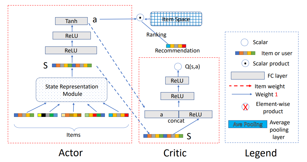
The Actor network

For a given user, the network accounts for generating an action a based on her state $s$. Let us explain the network from the input to the output part. In DRR, the user state, denoted by the embeddings of her $n$ latest positively interacted items, is regarded as the input. Then the embeddings are fed into a state representation module to produce a summarized representation $s$ for the user. For instance, at timestep $t$, the state can be defined as $s_t = f(H_t)$ where $f(·)$ stands for the state representation module, $H_t = \{i_1, ..., i_n\}$ denotes the embeddings of the latest positive interaction history, and $i_t ∈ R^{1×k}$ is a $k$-dimensional vector.

When the recommender agent recommends an item $i_t$, if the user provides positive feedback, then in the next timestep, the state is updated to $s_{t+1} = f(H_{t+1})$, where $H_{t+1} = \{i_2, ..., i_n, i_t\}$; otherwise, $H_{t+1} = H_t$. The reasons to define the state in such a manner are two folds: (i) a superior recommender system should cater to the users’ taste, i.e., what items the users like; (ii) the latest records represent the users’ recent interests more precisely.

Finally, by two ReLU layers and one Tanh layer, the state representation s is transformed into an action $a = π_θ(s)$ as the output of the Actor network. Particularly, the action a is defined as a ranking function represented by a continuous parameter vector $a ∈ R^{1×k}$ . By using the action, the ranking score of the item it is defined as $score_t = i_ta^T$. Then, the top ranked item (w.r.t. the ranking scores) is recommended to the user. Note that, the widely used ε-greedy exploration technique is adopted here.

Implementation in Tensorflow

import tensorflow as tf
import numpy as np

class ActorNetwork(tf.keras.Model):
    def __init__(self, embedding_dim, hidden_dim):
        super(ActorNetwork, self).__init__()
        self.inputs = tf.keras.layers.InputLayer(name='input_layer', input_shape=(3*embedding_dim,))
        self.fc = tf.keras.Sequential([
            tf.keras.layers.Dense(hidden_dim, activation='relu'),
            tf.keras.layers.Dense(hidden_dim, activation='relu'),
            tf.keras.layers.Dense(embedding_dim, activation='tanh')
        ])
        
    def call(self, x):
        x = self.inputs(x)
        return self.fc(x)

class Actor(object):
    
    def __init__(self, embedding_dim, hidden_dim, learning_rate, state_size, tau):
        
        self.embedding_dim = embedding_dim
        self.state_size = state_size
        
        # actor network / target network
        self.network = ActorNetwork(embedding_dim, hidden_dim)
        self.target_network = ActorNetwork(embedding_dim, hidden_dim)
        # optimizer
        self.optimizer = tf.keras.optimizers.Adam(learning_rate)
        # soft target network update hyperparameter
        self.tau = tau
    
    def build_networks(self):
        # Build networks
        self.network(np.zeros((1, 3*self.embedding_dim)))
        self.target_network(np.zeros((1, 3*self.embedding_dim)))
    
    def update_target_network(self):
        # soft target network update
        c_theta, t_theta = self.network.get_weights(), self.target_network.get_weights()
        for i in range(len(c_theta)):
            t_theta[i] = self.tau * c_theta[i] + (1 - self.tau) * t_theta[i]
        self.target_network.set_weights(t_theta)
        
    def train(self, states, dq_das):
        with tf.GradientTape() as g:
            outputs = self.network(states)
            # loss = outputs*dq_das
        dj_dtheta = g.gradient(outputs, self.network.trainable_weights, -dq_das)
        grads = zip(dj_dtheta, self.network.trainable_weights)
        self.optimizer.apply_gradients(grads)
        
    def save_weights(self, path):
        self.network.save_weights(path)
        
    def load_weights(self, path):
        self.network.load_weights(path)

Implementation in PyTorch

class Actor(nn.Module):
    def __init__(self, in_features=100, out_features=18):
        super(Actor, self).__init__()
        self.in_features = in_features
        self.out_features = out_features

        self.linear1 = nn.Linear(self.in_features, self.in_features)
        self.linear2 = nn.Linear(self.in_features, self.in_features)
        self.linear3 = nn.Linear(self.in_features, self.out_features)

    def forward(self, state):
        output = F.relu(self.linear1(state))
        output = F.relu(self.linear2(output))
        output = F.tanh(self.linear3(output))
        return output

The Critic network

The Critic part in DRR is a Deep Q-Network, which leverages a deep neural network parameterized as $Q_ω(s, a)$ to approximate the true state-action value function $Q_π (s, a)$, namely, the Q-value function. The Q-value function reflects the merits of the action policy generated by the Actor network. Specifically, the input of the Critic network is the user state s generated by the user state representation module and the action a generated by the policy network, and the output is the Q-value, which is a scalar. According to the Q-value, the parameters of the Actor network are updated in the direction of improving the performance of action a, i.e., boosting $Q_ω(s, a)$.

Based on the deterministic policy gradient theorem, we can update the Actor by the sampled policy gradient $∇_θJ(π_θ) ≈ \dfrac{1}{N} \sum_t ∇_aQ_ω(s,a)|_{s=s_t,a=π_θ(s_t)}∇_θπ_θ(s)|_{s=s_t},$ where $J(π_θ)$ is the expectation of all possible Q-values that follow the policy $π_θ$. Here the mini-batch strategy is utilized and $N$ denotes the batch size. Moreover, the Critic network is updated accordingly by the temporal-difference learning approach, i.e., minimizing the mean squared error $L = \dfrac{1}{N}\sum_i(y_i − Q_ω(s_i,a_i))^2$ where $y_i = r_i + γQ_{ω'}(s_{i+1}, π_{θ'}(s_{i+1}))$. The target network technique is also adopted in DRR framework, where $ω'$ and $θ'$ is the parameters of the target Critic and Actor network.

Implementation in PyTorch

class Critic(nn.Module):
    def __init__(self, action_size=20, in_features=128, out_features=18):
        super(Critic, self).__init__()
        self.in_features = in_features
        self.out_features = out_features
        self.combo_features = in_features + action_size
        self.action_size = action_size

        self.linear1 = nn.Linear(self.in_features, self.in_features)
        self.linear2 = nn.Linear(self.combo_features, self.combo_features)
        self.linear3 = nn.Linear(self.combo_features, self.combo_features)
        self.output_layer = nn.Linear(self.combo_features, self.out_features)

    def forward(self, state, action):
        output = F.relu(self.linear1(state))
        output = torch.cat((action, output), dim=1)
        output = F.relu(self.linear2(output))
        output = F.relu(self.linear3(output))
        output = self.output_layer(output)
        return output

The State Representation Module

As noted above, the state representation module plays an important role in both the Actor network and Critic network. Hence, it is very crucial to design a good structure to model the state.

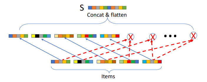
DRR-p Structure

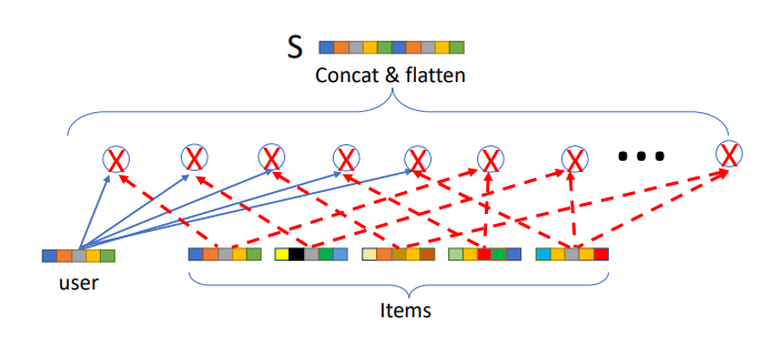
DRR-u Structure

DRR-ave Structure

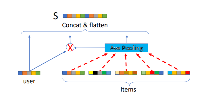
Implementation in PyTorch

class DRRAveStateRepresentation(nn.Module):
    def __init__(self, n_items=5, item_features=100, user_features=100):
        super(DRRAveStateRepresentation, self).__init__()
        self.n_items = n_items
        self.random_state = RandomState(1)
        self.item_features = item_features
        self.user_features = user_features

        self.attention_weights = nn.Parameter(torch.from_numpy(0.1 * self.random_state.rand(self.n_items)).float())

    def forward(self, user, items):
        '''
        DRR-AVE State Representation
        :param items: (torch tensor) shape = (n_items x item_features),
                Matrix of items in history buffer
        :param user: (torch tensor) shape = (1 x user_features),
                User embedding
        :return: output: (torch tensor) shape = (3 * item_features)
        '''
        right = items.t() @ self.attention_weights
        middle = user * right
        output = torch.cat((user, middle, right), 0).flatten()
        return output

Training Procedure of the DRR Framework

The training procedure mainly includes two phases, i.e., transition generation (lines 7-12) and model updating (lines 13-17).

For the first stage, the recommender observes the current state $s_t$ that is calculated by the proposed state representation module, then generates an action $a_t = π_θ(s_t)$ according to the current policy $π_θ$ with ε-greedy exploration, and recommends an item it according to the action $a_t$ (lines 8-9). Subsequently, the reward $r_t$ can be calculated based on the feedback of the user to the recommended item $i_t$, and the user state is updated (lines 10-11). Finally, the recommender agent stores the transition $(s_t, a_t, r_t, s_{t+1})$ into the replay buffer $D$ (line 12).

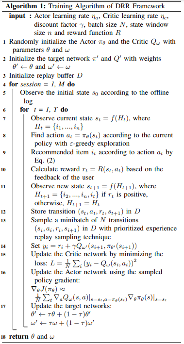
In the second stage, the model updating, the recommender samples a minibatch of $N$ transitions with widely used prioritized experience replay sampling technique (line 13), which is essentially an importance sampling strategy. Then, the recommender updates the parameters of the Actor network and Critic network respectively (line 14-16). Finally, the recommender updates the target networks’ parameters with the soft replace strategy.

Evaluation

The most straightforward way to evaluate the RL based models is to conduct online experiments on recommender systems where the recommender directly interacts with users. However, the underlying commercial risk and the costly deployment on the platform make it impractical. Therefore, throughout the testing phase, we conduct the evaluation of the proposed models on public offline datasets and propose two ways to evaluate the models, which are the offline evaluation and the online evaluation.

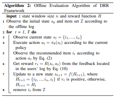
Offline evaluation

Intuitively, the offline evaluation of the trained models is to test the recommendation performance with the learned policy, which is described in Algorithm 2. Specifically, for a given session $S_j$ , the recommender only recommends the items that appear in this session, denoted as $I(S_j)$, rather than the ones in the whole item space. The reason is that we only have the ground truth feedback for the items in the session in the recorded offline log. For each timestep, the recommender agent takes an action at according to the learned policy $π_θ$, and recommends an item $i_t ∈ I(S_j)$ based on the action $a_t$ (lines 4-5). After that, the recommender observes the reward $r_t = R(s_t, a_t)$ according to the feedback of the recommended item $i_t$ (lines 5-6). Then the user state is updated to $s_{t+1}$ and the recommended item $i_t$ is removed from the candidate set $I(S_j)$ (lines 7-8). The offline evaluation procedure can be treated as a rerank procedure of the candidate set by iteratively selecting an item w.r.t. the action generated by the Actor network in DRR framework. Moreover, the model parameters are not updated in the offline evaluation.

Online evaluation with environment simulator

As aforementioned that it is risky and costly to directly deploy the RL based models on recommender systems. Therefore, we can conduct online evaluation with an environment simulator. We basically pretrain a PMF model as the environment simulator, i.e., to predict an item’s feedback that the user never rates before. The online evaluation procedure follows Algorithm 1, i.e., the parameters continuously update during the online evaluation stage. Its major difference from Algorithm 1 is that the feedback of a recommended item is observed by the environment simulator. Moreover, before each recommendation session starting in the simulated online evaluation, we reset the parameters back to θ and ω which is the policy learned in the training stage for a fair comparison.