BPR

BPR stands for Bayesian Personalized Ranking. In matrix factorization (MF), to compute the prediction we have to multiply the user factors to the item factors:

\hat{x}_{ui} = \langle w_u,h_i \rangle = \sum_{f=1}^k w_{uf} \cdot h_{if}

The usual approach for item recommenders is to predict a personalized score $\hat{x}_{ui}$ for an item that reflects the preference of the user for the item. Then the items are ranked by sorting them according to that score. Machine learning approaches are typically fit by using observed items as a positive sample and missing ones for the negative class. A perfect model would thus be useless, as it would classify as negative (non-interesting) all the items that were non-observed at training time. The only reason why such methods work is regularization.

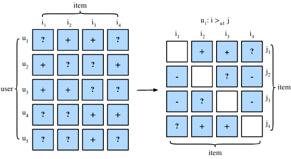
BPR use a different approach. The training dataset is composed by triplets $(u,i,j)$ representing that user $u$ is assumed to prefer $i$ over $j$ . For an implicit dataset this means that $u$ observed $i$ but not $j$ :

D_S := \{(u,i,j) \mid i \in I_u^+ \wedge j \in I \setminus I_u^+\}

A machine learning model can be represented by a parameter vector $Θ$ which is found at fitting time. BPR wants to find the parameter vector that is most probable given the desired, but latent, preference structure $>_u$ :

\begin{align} p(\Theta \mid >_u) \propto p(>_u \mid \Theta)p(\Theta) \\ \prod_{u\in U} p(>_u \mid \Theta) = \dots = \prod_{(u,i,j) \in D_S} p(i >_u j \mid \Theta) \end{align}

The probability that a user really prefers item $i$ to item $j$ is defined as:

\begin{align} p(i >_u j \mid \Theta) := \sigma(\hat{x}_{uij}(\Theta)) \end{align}

Where $σ$ represent the logistic sigmoid and $\hat{x}_{uij}(Θ)$ is an arbitrary real-valued function of $Θ$ (the output of your arbitrary model).

User $u_1$ has interacted with item $i_2$ but not item $i_1$ , so we assume that this user prefers item $i_2$ over $i_1$ . For items that the user have both interacted with, we cannot infer any preference. The same is true for two items that a user has not interacted yet (e.g. item $i_1$ and $i_4$ for user $u_1$ ).

/img/content-models-raw-mp2-bpr-untitled.png

To complete the Bayesian setting, we define a prior density for the parameters:

p(\Theta) \sim N(0, \Sigma_\Theta)

And we can now formulate the maximum posterior estimator:

\begin{equation} \begin{split} BPR-OPT &=\log p(\Theta \mid >_u)\\ &=\log p(>_u \mid \Theta) p(\Theta) \\ &= \log \prod_{(u,i,j) \in D_S} \sigma(\hat{x}_{uij})p(\Theta) \\ &= \sum_{(u,i,j) \in D_S} \log \sigma(\hat{x}_{uij}) + \log p(\Theta) \\ &= \sum_{(u,i,j) \in D_S} \log \sigma(\hat{x}_{uij}) - \lambda_\Theta ||\Theta||^2 \end{split} \end{equation}

Where $λ_Θ$ are model specific regularization parameters.

Once obtained the log-likelihood, we need to maximize it in order to find our optimal $Θ$ . As the criterion is differentiable, gradient descent algorithms are an obvious choiche for maximization.

The basic version of gradient descent consists in evaluating the gradient using all the available samples and then perform a single update. The problem with this is, in our case, that our training dataset is very skewed. Suppose an item $i$ is very popular. Then we have many terms of the form $\hat{x}_{uij}$ in the loss because for many users $u$ the item $i$ is compared against all negative items $j$ . The other popular approach is stochastic gradient descent, where for each training sample an update is performed. This is a better approach, but the order in which the samples are traversed is crucial. To solve this issue BPR uses a stochastic gradient descent algorithm that chooses the triples randomly.

The gradient of BPR-OPT with respect to the model parameters is:

\begin{equation} \begin{split} \frac{\partial BPR-OPT}{\partial \Theta} &= \sum_{(u,i,j) \in D_S} \frac{\partial}{\partial \Theta} \log \sigma (\hat{x}_{uij}) - \lambda_\Theta \frac{\partial}{\partial\Theta} || \Theta ||^2\\ &= \sum_{(u,i,j) \in D_S} \frac{-e^{-\hat{x}_{uij}}}{1+e^{-\hat{x}_{uij}}} \frac{\partial}{\partial \Theta}\hat{x}_{uij} - \lambda_\Theta \Theta \end{split} \end{equation}

In order to practically apply this learning schema to an existing algorithm, we first split the real valued preference term: $\hat{x}_{uij} := \hat{x}_{ui} − \hat{x}_{uj}$ . And now we can apply any standard collaborative filtering model that predicts $\hat{x}_{ui}$ .

The problem of predicting $\hat{x}_{ui}$ can be seen as the task of estimating a matrix $X:U×I$ . With matrix factorization the target matrix $X$ is approximated by the matrix product of two low-rank matrices $W:|U|×k$ and $H:|I|×k$ :

X := WH^t

The prediction formula can also be written as:

\hat{x}_{ui} = \langle w_u,h_i \rangle = \sum_{f=1}^k w_{uf} \cdot h_{if}

Besides the dot product ⟨⋅,⋅⟩, in general any kernel can be used.

We can now specify the derivatives:

\frac{\partial}{\partial \theta} \hat{x}_{uij} = \begin{cases} (h_{if} - h_{jf}) \text{ if } \theta=w_{uf}, \\ w_{uf} \text{ if } \theta = h_{if}, \\ -w_{uf} \text{ if } \theta = h_{jf}, \\ 0 \text{ else } \end{cases}

Which basically means: user $u$ prefer $i$ over $j$ , let's do the following:

Increase the relevance (according to $u$ ) of features belonging to $i$ but not to $j$ and vice-versa
Increase the relevance of features assigned to $i$
Decrease the relevance of features assigned to $j$

BPR

Links​

Links