FFM
FFM stands for Field-aware Factorization Machines. In the official FFM paper, it is empirically proven that for large, sparse datasets with many categorical features, FFM performs better. Conversely, for small and dense datasets or numerical datasets, FFM may not be as effective as FM. FFM is also prone to overfitting on the training dataset, hence one should use a standalone validation set and use early stopping when the loss increases.
research paper
Yuchin Juan et al. “Field-aware Factorization Machines for CTR Prediction” in RecSys 2016.
Click-through rate (CTR) prediction plays an important role in computational advertising. Models based on degree-2 polynomial mappings and factorization machines (FMs) are widely used for this task. Recently, a variant of FMs, field-aware factorization machines (FFMs), outperforms existing models in some world-wide CTR-prediction competitions. Based on our experiences in winning two of them, in this paper we establish FFMs as an effective method for classifying large sparse data including those from CTR prediction. First, we propose efficient implementations for training FFMs. Then we comprehensively analyze FFMs and compare this approach with competing models. Experiments show that FFMs are very useful for certain classification problems. Finally, we have released a package of FFMs for public use.
Despite effectiveness, FM can be hindered by its modelling of all feature interactions with the same weight, as not all feature interactions are equally useful and predictive. For example, the interactions with useless features may even introduce noises and adversely degrade the performance.
| For each | Learn | |
|---|---|---|
| Linear | feature | a weight |
| Poly | feature pair | a weight |
| FM | feature | a latent vector |
| FFM | feature | multiple latent vectors |
Field-aware factorization machine (FFM) is an extension to FM. It was originally introduced in [2]. The advantage of FFM over FM is that it uses different factorized latent factors for different groups of features. The "group" is called "field" in the context of FFM. Putting features into fields resolves the issue that the latent factors shared by features that intuitively represent different categories of information may not well generalize the correlation.
Assume we have the following dataset where we want to predict Clicked outcome using Publisher, Advertiser, and Gender:
| Dataset | Clicked | Publisher | Advertiser | Gender |
|---|---|---|---|---|
| Train | Yes | ESPN | Nike | Male |
| Train | No | NBC | Adidas | Male |
The model for logistic regression, Poly2, FM, and FFM, is obtained by solving the following optimization problem:
where,
- dataset contains instances
- is the label and is a -dimensional feature vector
- λ is a regularization parameter
- is the association between and
Here is the comparison of different models:
Linear Regression
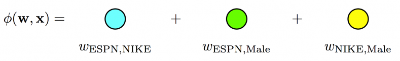
A logistic regression estimates the outcome by learning the weight for each feature.
In our context:
Degree-2 Polynomial Mappings (Poly2)
A Poly2 model captures this pair-wise feature interaction by learning a dedicated weight for each feature pair.
In our context:
Poly2 model - A dedicated weight is learned for each feature pair (linear terms ignored in diagram).
However, a Poly2 model is computationally expensive as it requires the computation of all feature pair combinations. Also, when data is sparse, there might be some unseen pairs in the test set.
Factorization Machines
FM solves this problem by learning the pairwise feature interactions in a latent space. Each feature has an associated latent vector. The interaction between two features is an inner-product of their respective latent vectors.
In our context:
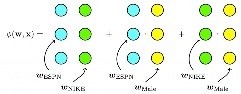
Factorization Machines - Each feature has one latent vector, which is used to interact with any other latent vectors (linear terms ignored in diagram).
Field-aware Factorization Machines
FFM addresses this issue by splitting the original latent space into smaller latent spaces specific to the fields of the features.
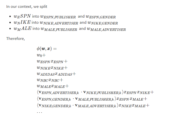
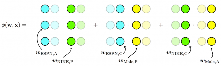
Field-aware Factorization Machines - Each feature has several latent vectors, one of them is used depending on the field of the other feature (linear terms ignored in diagram).
Links
- https://wngaw.github.io/field-aware-factorization-machines-with-xlearn
- https://www.csie.ntu.edu.tw/~cjlin/papers/ffm.pdf
- https://dl.acm.org/doi/pdf/10.1145/2959100.2959134
- https://github.com/rixwew/pytorch-fm
- https://github.com/PaddlePaddle/PaddleRec/blob/release/2.1.0/models/rank/ffm
- https://recbole.io/docs/recbole/recbole.model.context_aware_recommender.ffm.html
- https://towardsdatascience.com/an-intuitive-explanation-of-field-aware-factorization-machines-a8fee92ce29f
- https://medium.com/@vinitvssingh5/explaining-the-field-aware-factorization-machines-ffms-for-ctr-prediction-2e98b2949dd6
- https://ailab.criteo.com/ctr-prediction-linear-model-field-aware-factorization-machines/