CartPole using Cross-Entropy¶

Despite the fact that it is much less famous than other tools in the RL practitioner’s toolbox, such as deep Q-network (DQN) or advantage actor-critic, the cross-entropy method has its own strengths. Firstly, the cross-entropy method is really simple, which makes it an easy method to follow. For example, its implementation on PyTorch is less than 100 lines of code.

Secondly, the method has good convergence. In simple environments that don’t require complex, multistep policies to be learned and discovered, and that have short episodes with frequent rewards, the cross-entropy method usually works very well. Of course, lots of practical problems don’t fall into this category, but sometimes they do. In such cases, the cross-entropy method (on its own or as part of a larger system) can be the perfect fit.

Cross-entropy method is model-free, policy-based, and on-policy, which means the following:

It doesn’t build any model of the environment; it just says to the agent what to do at every step
It approximates the policy of the agent
It requires fresh data obtained from the environment

import gym
from collections import namedtuple
import numpy as np
from torch.utils.tensorboard import SummaryWriter

import torch
import torch.nn as nn
import torch.optim as optim

We define constants and they include the count of neurons in the hidden layer, the count of episodes we play on every iteration, and the percentile of episodes’ total rewards that we use for “elite” episode filtering. We will take the 70th percentile, which means that we will leave the top 30% of episodes sorted by reward.

HIDDEN_SIZE = 128
BATCH_SIZE = 16
PERCENTILE = 70

Our model’s core is a one-hidden-layer NN, with rectified linear unit (ReLU) and 128 hidden neurons (which is absolutely arbitrary). Other hyperparameters are also set almost randomly and aren’t tuned, as the method is robust and converges very quickly.

class Net(nn.Module):
    def __init__(self, obs_size, hidden_size, n_actions):
        super(Net, self).__init__()
        self.net = nn.Sequential(
            nn.Linear(obs_size, hidden_size),
            nn.ReLU(),
            nn.Linear(hidden_size, n_actions)
        )

    def forward(self, x):
        return self.net(x)

There is nothing special about our NN; it takes a single observation from the environment as an input vector and outputs a number for every action we can perform. The output from the NN is a probability distribution over actions, so a straightforward way to proceed would be to include softmax nonlinearity after the last layer. However, in the preceding NN, we don’t apply softmax to increase the numerical stability of the training process. Rather than calculating softmax (which uses exponentiation) and then calculating cross-entropy loss (which uses a logarithm of probabilities), we can use the PyTorch class nn.CrossEntropyLoss, which combines both softmax and cross-entropy in a single, more numerically stable expression. CrossEntropyLoss requires raw, unnormalized values from the NN (also called logits). The downside of this is that we need to remember to apply softmax every time we need to get probabilities from our NN’s output.

Episode = namedtuple('Episode', field_names=['reward', 'steps'])
EpisodeStep = namedtuple('EpisodeStep', field_names=['observation', 'action'])

Here we will define two helper classes that are named tuples from the collections package in the standard library:

EpisodeStep: This will be used to represent one single step that our agent made in the episode, and it stores the observation from the environment and what action the agent completed. We will use episode steps from “elite” episodes as training data.
Episode: This is a single episode stored as total undiscounted reward and a collection of EpisodeStep.

Let’s look at a function that generates batches with episodes:

def iterate_batches(env, net, batch_size):
    batch = []
    episode_reward = 0.0
    episode_steps = []
    obs = env.reset()
    sm = nn.Softmax(dim=1)
    while True:
        obs_v = torch.FloatTensor([obs])
        act_probs_v = sm(net(obs_v))
        act_probs = act_probs_v.data.numpy()[0]
        action = np.random.choice(len(act_probs), p=act_probs)
        next_obs, reward, is_done, _ = env.step(action)
        episode_reward += reward
        step = EpisodeStep(observation=obs, action=action)
        episode_steps.append(step)
        if is_done:
            e = Episode(reward=episode_reward, steps=episode_steps)
            batch.append(e)
            episode_reward = 0.0
            episode_steps = []
            next_obs = env.reset()
            if len(batch) == batch_size:
                yield batch
                batch = []
        obs = next_obs

The preceding function accepts the environment (the Env class instance from the Gym library), our NN, and the count of episodes it should generate on every iteration. The batch variable will be used to accumulate our batch (which is a list of Episode instances). We also declare a reward counter for the current episode and its list of steps (the EpisodeStep objects). Then we reset our environment to obtain the first observation and create a softmax layer, which will be used to convert the NN’s output to a probability distribution of actions. That’s our preparations complete, so we are ready to start the environment loop.

At every iteration, we convert our current observation to a PyTorch tensor and pass it to the NN to obtain action probabilities. There are several things to note here:

All nn.Module instances in PyTorch expect a batch of data items and the same is true for our NN, so we convert our observation (which is a vector of four numbers in CartPole) into a tensor of size 1×4 (to achieve this, we pass an observation in a single-element list).
As we haven’t used nonlinearity at the output of our NN, it outputs raw action scores, which we need to feed through the softmax function.
Both our NN and the softmax layer return tensors that track gradients, so we need to unpack this by accessing the tensor.data field and then converting the tensor into a NumPy array. This array will have the same two-dimensional structure as the input, with the batch dimension on axis 0, so we need to get the first batch element to obtain a one-dimensional vector of action probabilities.

Now that we have the probability distribution of actions, we can use it to obtain the actual action for the current step by sampling this distribution using NumPy’s function random.choice(). After this, we will pass this action to the environment to get our next observation, our reward, and the indication of the episode ending.

The reward is added to the current episode’s total reward, and our list of episode steps is also extended with an (observation, action) pair. Note that we save the observation that was used to choose the action, but not the observation returned by the environment as a result of the action. These are the tiny, but important, details that you need to keep in mind.

This is how we handle the situation when the current episode is over (in the case of CartPole, the episode ends when the stick has fallen down despite our efforts). We append the finalized episode to the batch, saving the total reward (as the episode has been completed and we have accumulated all the reward) and steps we have taken. Then we reset our total reward accumulator and clean the list of steps. After that, we reset our environment to start over.

In case our batch has reached the desired count of episodes, we return it to the caller for processing using yield. Our function is a generator, so every time the yield operator is executed, the control is transferred to the outer iteration loop and then continues after the yield line. If you are not familiar with Python’s generator functions, refer to the Python documentation: https://wiki.python.org/moin/Generators. After processing, we will clean up the batch.

The last, but very important, step in our loop is to assign an observation obtained from the environment to our current observation variable. After that, everything repeats infinitely—we pass the observation to the NN, sample the action to perform, ask the environment to process the action, and remember the result of this processing.

One very important fact to understand in this function logic is that the training of our NN and the generation of our episodes are performed at the same time. They are not completely in parallel, but every time our loop accumulates enough episodes (16), it passes control to this function caller, which is supposed to train the NN using gradient descent. So, when yield is returned, the NN will have different, slightly better (we hope) behavior.

We don’t need to explore proper synchronization, as our training and data gathering activities are performed at the same thread of execution, but you need to understand those constant jumps from NN training to its utilization.

Okay, now we need to define yet another function and then we will be ready to switch to the training loop.

def filter_batch(batch, percentile):
    rewards = list(map(lambda s: s.reward, batch))
    reward_bound = np.percentile(rewards, percentile)
    reward_mean = float(np.mean(rewards))

    train_obs = []
    train_act = []
    for reward, steps in batch:
        if reward < reward_bound:
            continue
        train_obs.extend(map(lambda step: step.observation, steps))
        train_act.extend(map(lambda step: step.action, steps))

    train_obs_v = torch.FloatTensor(train_obs)
    train_act_v = torch.LongTensor(train_act)
    return train_obs_v, train_act_v, reward_bound, reward_mean

This function is at the core of the cross-entropy method—from the given batch of episodes and percentile value, it calculates a boundary reward, which is used to filter “elite” episodes to train on. To obtain the boundary reward, we will use NumPy’s percentile function, which, from the list of values and the desired percentile, calculates the percentile’s value. Then, we will calculate the mean reward, which is used only for monitoring.

Next, we will filter off our episodes. For every episode in the batch, we will check that the episode has a higher total reward than our boundary and if it has, we will populate lists of observations and actions that we will train on.

As the final step of the function, we will convert our observations and actions from “elite” episodes into tensors, and return a tuple of four: observations, actions, the boundary of reward, and the mean reward. The last two values will be used only to write them into TensorBoard to check the performance of our agent.

Now, the final chunk of code that glues everything together, and mostly consists of the training loop, is as follows:

if __name__ == "__main__":
    env = gym.make("CartPole-v0")
    # env = gym.wrappers.Monitor(env, directory="mon", force=True)
    obs_size = env.observation_space.shape[0]
    n_actions = env.action_space.n

    net = Net(obs_size, HIDDEN_SIZE, n_actions)
    objective = nn.CrossEntropyLoss()
    optimizer = optim.Adam(params=net.parameters(), lr=0.01)
    writer = SummaryWriter(comment="-cartpole")

    for iter_no, batch in enumerate(iterate_batches(
            env, net, BATCH_SIZE)):
        obs_v, acts_v, reward_b, reward_m = \
            filter_batch(batch, PERCENTILE)
        optimizer.zero_grad()
        action_scores_v = net(obs_v)
        loss_v = objective(action_scores_v, acts_v)
        loss_v.backward()
        optimizer.step()
        print("%d: loss=%.3f, reward_mean=%.1f, rw_bound=%.1f" % (
            iter_no, loss_v.item(), reward_m, reward_b))
        writer.add_scalar("loss", loss_v.item(), iter_no)
        writer.add_scalar("reward_bound", reward_b, iter_no)
        writer.add_scalar("reward_mean", reward_m, iter_no)
        if reward_m > 199:
            print("Solved!")
            break
    writer.close()

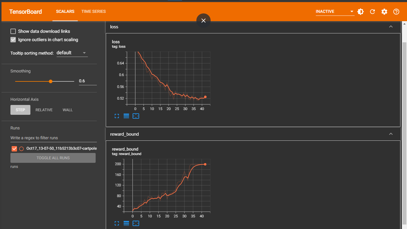
loss=0.695, reward_mean=20.1, rw_bound=23.5
loss=0.681, reward_mean=32.9, rw_bound=36.5
loss=0.667, reward_mean=28.1, rw_bound=31.0
loss=0.660, reward_mean=33.0, rw_bound=36.5
loss=0.639, reward_mean=37.6, rw_bound=48.5
loss=0.641, reward_mean=48.1, rw_bound=49.5
loss=0.633, reward_mean=53.8, rw_bound=52.5
loss=0.609, reward_mean=59.6, rw_bound=66.0
loss=0.615, reward_mean=49.8, rw_bound=50.0
loss=0.600, reward_mean=65.1, rw_bound=78.0
loss=0.586, reward_mean=56.9, rw_bound=71.0
loss=0.599, reward_mean=68.3, rw_bound=77.0
loss=0.589, reward_mean=60.6, rw_bound=67.5
loss=0.586, reward_mean=61.2, rw_bound=72.5
loss=0.571, reward_mean=64.5, rw_bound=70.5
loss=0.562, reward_mean=68.9, rw_bound=84.0
loss=0.572, reward_mean=60.4, rw_bound=61.5
loss=0.563, reward_mean=87.5, rw_bound=91.0
loss=0.548, reward_mean=81.9, rw_bound=89.0
loss=0.575, reward_mean=91.8, rw_bound=99.0
loss=0.544, reward_mean=71.1, rw_bound=68.5
loss=0.528, reward_mean=78.4, rw_bound=85.5
loss=0.539, reward_mean=87.1, rw_bound=89.5
loss=0.517, reward_mean=83.2, rw_bound=91.5
loss=0.545, reward_mean=95.3, rw_bound=99.0
loss=0.532, reward_mean=94.1, rw_bound=103.5
loss=0.535, reward_mean=114.5, rw_bound=131.5
loss=0.530, reward_mean=112.2, rw_bound=134.0
loss=0.523, reward_mean=118.9, rw_bound=134.5
loss=0.540, reward_mean=133.2, rw_bound=154.0
loss=0.517, reward_mean=135.7, rw_bound=173.0
loss=0.537, reward_mean=124.8, rw_bound=154.5
loss=0.518, reward_mean=122.4, rw_bound=139.0
loss=0.515, reward_mean=170.8, rw_bound=193.5
loss=0.530, reward_mean=164.8, rw_bound=200.0
loss=0.515, reward_mean=176.1, rw_bound=200.0
loss=0.526, reward_mean=194.8, rw_bound=200.0
loss=0.514, reward_mean=185.1, rw_bound=200.0
loss=0.513, reward_mean=179.2, rw_bound=200.0
loss=0.526, reward_mean=195.6, rw_bound=200.0
loss=0.523, reward_mean=196.6, rw_bound=200.0
loss=0.520, reward_mean=195.2, rw_bound=200.0
loss=0.532, reward_mean=199.4, rw_bound=200.0
Solved!

In the training loop, we iterate our batches (a list of Episode objects), then we perform filtering of the “elite” episodes using the filter_batch function. The result is variables of observations and taken actions, the reward boundary used for filtering, and the mean reward. After that, we zero gradients of our NN and pass observations to the NN, obtaining its action scores. These scores are passed to the objective function, which will calculate cross-entropy between the NN output and the actions that the agent took. The idea of this is to reinforce our NN to carry out those “elite” actions that have led to good rewards. Then, we calculate gradients on the loss and ask the optimizer to adjust our NN.

The rest of the loop is mostly the monitoring of progress. On the console, we show the iteration number, the loss, the mean reward of the batch, and the reward boundary. We also write the same values to TensorBoard, to get a nice chart of the agent’s learning performance.

The last check in the loop is the comparison of the mean rewards of our batch episodes. When this becomes greater than 199, we stop our training. Why 199? In Gym, the CartPole environment is considered to be solved when the mean reward for the last 100 episodes is greater than 195, but our method converges so quickly that 100 episodes are usually what we need. The properly trained agent can balance the stick infinitely long (obtaining any amount of score), but the length of an episode in CartPole is limited to 200 steps (if you look at the environment variable of CartPole, you may notice the TimeLimit wrapper, which stops the episode after 200 steps). With all this in mind, we will stop training after the mean reward in the batch is greater than 199, which is a good indication that our agent knows how to balance the stick like a pro.

%load_ext tensorboard

%tensorboard --logdir runs

drl-recsys

CartPole using Cross-Entropy¶