Deep Reinforcement Learning in Recommendation Systems
The idea that we learn by interacting with our environment is probably the first to occur to us when we think about the nature of learning. When an infant plays, waves its arms, or looks about, it has no explicit teacher, but it does have a direct sensorimotor connection to its environment. Exercising this connection produces a wealth of information about cause and effect, about the consequences of actions, and about what to do in order to achieve goals. Throughout our lives, such interactions are undoubtedly a major source of knowledge about our environment and ourselves. Whether we are learning to drive a car or to hold a conversation, we are acutely aware of how our environment responds to what we do, and we seek to influence what happens through our behavior. Learning from interaction is a foundational idea underlying nearly all theories of learning and intelligence.
Reinforcement learning is learning what to do—how to map situations to actions—so as to maximize a numerical reward signal. The learner is not told which actions to take, but instead must discover which actions yield the most reward by trying them. In the most interesting and challenging cases, actions may affect not only the immediate reward but also the next situation and, through that, all subsequent rewards. These two characteristics—trial-and-error search and delayed reward—are the two most important distinguishing features of reinforcement learning.
According to Sutton and Barto, three characteristics distinguish an RL problem: (1) the problem is closed-loop, (2) the learner does not have a tutor to teach it what to do, but it should figure out what to do through trial-and-error, and (3) actions influence not only the short term results, but also the long-term ones. Let’s suppose we are teaching a dog (agent) to catch a ball. Instead of teaching the dog explicitly to catch a ball, we just throw a ball and every time the dog catches the ball, we give the dog a cookie (reward). If the dog fails to catch the ball, then we do not give it a cookie. So, the dog will figure out what action caused it to receive a cookie and repeat that action. Thus, the dog will understand that catching the ball caused it to receive a cookie and will attempt to repeat catching the ball. Thus, in this way, the dog will learn to catch a ball while aiming to maximize the cookies it can receive.
Similarly, in an RL setting, we will not teach the agent what to do or how to do it; instead, we will give a reward to the agent for every action it does. We will give a positive reward to the agent when it performs a good action and we will give a negative reward to the agent when it performs a bad action. The agent begins by performing a random action and if the action is good, we then give the agent a positive reward so that the agent understands it has performed a good action and it will repeat that action. If the action performed by the agent is bad, then we will give the agent a negative reward so that the agent will understand it has performed a bad action and it will not repeat that action.
Overview
The early history of reinforcement learning has two main threads, both long and rich, that were pursued independently before intertwining in modern reinforcement learning. One thread concerns learning by trial and error that started in the psychology of animal learning. This thread runs through some of the earliest work in artificial intelligence and led to the revival of reinforcement learning in the early 1980s. The other thread concerns the problem of optimal control and its solution using value functions and dynamic programming. For the most part, this thread did not involve learning. Although the two threads have been largely independent, the exceptions revolve around a third, less distinct thread concerning temporal-difference methods. All three threads came together in the late 1980s to produce the modern field of reinforcement learning. So technically, the foundation of reinforcement learning (RL) is based upon three topics. The most important is the Markov decision process (MDP), a framework that helps you describe your problem. Dynamic programming (DP) and Monte Carlo methods lie at the heart of all algorithms that intend to solve MDPs.
In the MC method, to compute the value of a state, we generate some N trajectories and compute the value of a state as an average return of a state across the N trajectories. We learned that when the trajectory is too long, then the MC method will take us a lot of time to compute the value of the state and is also unsuitable for non-episodic tasks. So, we resorted to the TD learning method. In the TD learning method, we learned that instead of waiting until the end of the episode to compute the value of the state, we can make use of bootstrapping and estimate the value of the state as the sum of the immediate reward and the discounted value of the next state.
RL is one of the most active areas of research in artificial intelligence, and it is believed that RL will take us a step closer towards achieving artificial general intelligence. RL has evolved rapidly in the past few years with a wide variety of applications ranging from building a recommendation system to self-driving cars. The major reason for this evolution is the advent of deep reinforcement learning, which is a combination of deep learning and RL. With the emergence of new RL algorithms and libraries, RL is clearly one of the most promising areas of ML.
RL problems can be expressed as a system consisting of an agent and an environment. An environment produces information which describes the state of the system. This is known as a state. An agent interacts with an environment by observing the state and using this information to select an action. We call an agent’s action-producing function a policy. Formally, a policy is a function which maps states to actions. An action will change the environment and affect what an agent observes and does next. RL problems have an objective, which is the sum of rewards received by an agent. An agent’s goal is to maximize the objective by selecting good actions. It learns to do this by interacting with the environment in a process of trial and error, and uses the reward signals it receives to reinforce good actions.
Essentially, a reinforcement learning system is a feedback control loop where an agent and an environment interact and exchange signals, while the agent tries to maximize the objective. The signals exchanged are ( \(s_t, a_t, r_t\)), which stand for the state, action, and reward, respectively, and t denotes the time step in which these signals occurred. The (\(s_t, a_t, r_t\)) tuple is called an experience. The control loop can repeat forever or terminate by reaching either a terminal state or a maximum time step t = T. The time horizon from t = 0 to when the environment terminates is called an episode. A trajectory is a sequence of experiences over an episode, τ = (\(s_0, a_0, r_0\)), (\(s_1, a_1, r_1\)), …. An agent typically needs many episodes to learn a good policy, ranging from hundreds to millions depending on the complexity of the problem.
The state-space 𝒮 is the set of all possible states in an environment. Depending on the environment, it can be defined in many different ways—as integers, real numbers, vectors, matrices, structured or unstructured data. Similarly, the action space 𝒜 is the set of all possible actions defined by an environment. It can also take many forms but is commonly defined as either a scalar or a vector. The reward function ℛ(\(s_t, a_t, s_{t+1}\)) assigns a positive, negative, or zero scalar to each transition (\(s_t, a_t, s_{t+1}\)).
Why is the goal of the agent to maximize the expected cumulative reward? Well, Reinforcement Learning is based on the idea of the reward hypothesis. All goals can be described by the maximization of the expected cumulative reward. That’s why in Reinforcement Learning, to have the best behavior, we need to maximize the expected cumulative reward.
The goal of the RL agent is to find a policy \(π(a|s)\) that takes action \(a ∈ \mathcal{A}\) in state \(s ∈ \mathcal{S}\) in order to maximize the expected, discounted cumulative reward \(max\ \mathbb{E}[R(τ)]\), where,
Model-Free or Model-Based
Model-based algorithms use definitive knowledge of the environment they are operating in to improve learning. For example, board games often limit the moves that you can make, and you can use this knowledge to (a) constrain the algorithm so that it does not provide invalid actions and (b) improve performance by projecting forward in time (for example, if I move here and if the opponent moves there, I can win). Human-beating algorithms for games like Go and poker can take advantage of the game’s fixed rules. You and your opponent can make a limited set of moves. This limits the number of strategies the algorithms have to search through. Like expert systems, model-based solutions learn efficiently because they don’t waste time searching improper paths.
Model-free algorithms can, in theory, apply to any problem. They learn strategies through interaction, absorbing any environmental rules in the process.
This is not the end of the story, however. Some algorithms can learn models of the environment at the same time as learning optimal strategies. Several new algorithms can also leverage the potential, but unknown actions of other agents (or other players). In other words, these agents can learn to counteract another agent’s strategies.
Algorithms such as these tend to blur the distinction between model-based and model-free, because ultimately you need a model of the environment somewhere. The difference is whether you can statically define it, whether you can learn it, or whether you can assume the model from the strategy.
Methods
Many algorithms have been proposed to solve an RL problem; they can be generally divided into tabular and approximate methods.
In tabular methods, value functions can be represented as tables, since the size of action and state spaces is small, so that exact optimal policy can be found. Popular tabular methods include dynamic programming (DP), Monte Carlo (MC), and temporal difference (TD). DP methods assume a perfect model of the environment and use a value function to search for good policies. Two important algorithms from this class are policy iteration and value iteration. Unlike DP, MC methods do not need a complete knowledge assumption about the environment. They only need a sample sequence of states, actions, and rewards from the environment, which could be real or simulated. Monte Carlo Tree Search (MCTS) is an important algorithm from this family. Moreover, TD methods are a combination of DP and MC methods. While they do not need a model from environment, they can bootstrap, which is the ability to update estimates based on other estimates. From this family, Q-learning, which is an off-policy algorithm and simply one of the most popular RL algorithms ever, and SARSA, an on-policy method, are very popular.
On the other hand, in approximate methods, since the size of state space is enormous, the goal is to find a good approximate solution with the constraint of limited computational resources. In approximate methods, a practical approach is to generalize from previous experiences (already seen states) to unseen states. Function approximation is the type of generalization required in RL and many techniques could be used to approximate the function, including artificial neural networks. Among the approximate solutions, policy gradient methods have been very popular, which learn a parameterized policy and can select actions without the need to a value function. REINFORCE and actor-critic are two important methods in this family. DL, which is based on artificial neural networks, has recently gained the attention of researchers in many fields due to their superior performance. This astonishing success inspired researchers at Google DeepMind to use DL as the function approximator in RL and propose deep Q-network (DQN), which is an approximate method for Q-learning. Later in deep deterministic policy gradient (DDPG), they extended this idea for continuous spaces, which is a combination of DQN and deterministic policy gradient (DPG). Other popular DRL methods used by RS community are double DQN (DDQN) and dueling Q-network.
Recent progress
There were other successes in the 2000s, but the field of DRL really only started growing after the DL field took off around 2010. In 2013 and 2015, Mnih et al. published a couple of papers presenting the DQN algorithm. DQN learned to play Atari games from raw pixels. Using a convolutional neural network (CNN) and a single set of hyperparameters, DQN performed better than a professional human player in 22 out of 49 games.
This accomplishment started a revolution in the DRL community: In 2014, Silver et al. released the deterministic policy gradient (DPG) algorithm, and a year later Lillicrap et al. improved it with deep deterministic policy gradient (DDPG). In 2016, Schulman et al. released trust region policy optimization (TRPO) and generalized advantage estimation (GAE) methods, Sergey Levine et al. published Guided Policy Search (GPS), and Silver et al. demoed AlphaGo. The following year, Silver et al. demonstrated AlphaZero. Many other algorithms were released during these years: double deep Q-networks (DDQN), prioritized experience replay (PER), proximal policy optimization (PPO), actor-critic with experience replay (ACER), asynchronous advantage actor-critic (A3C), advantage actor-critic (A2C), actor-critic using Kronecker-factored trust region (ACKTR), Rainbow, Unicorn (these are actual names, BTW), and so on. In 2019, Oriol Vinyals et al. showed the AlphaStar agent beat professional players at the game of StarCraft II. And a few months later, Jakub Pachocki et al. saw their team of Dota-2-playing bots, called Five, become the first AI to beat the world champions in an esports game.
Thanks to the progress in DRL, we’ve gone in two decades from solving backgammon, with its \(10^{20}\) perfect-information states, to solving the game of Go, with its \(10^{170}\) perfect-information states, or better yet, to solving StarCraft II, with its \(10^{270}\) imperfect-information states. It’s hard to conceive a better time to enter the field. Can you imagine what the next two decades will bring us? Will you be part of it? DRL is a booming field, and I expect its rate of progress to continue.
RL in Recommender systems
Recommender systems (RSs) are becoming an inseparable part of our everyday lives. They help us find our favorite items to purchase, our friends on social networks, and our favorite movies to watch. Traditionally, the recommendation problem was considered as a simple classification or prediction problem; however, the sequential nature of the recommendation problem has been shown.
Numerous techniques have been proposed to tackle the recommendation problem; traditional techniques include collaborative filtering, content-based filtering, and hybrid methods. Despite some success in providing relevant recommendations, specifically after the introduction of matrix factorization, these methods have severe problems, such as cold start, serendipity, scalability, low quality recommendation, and great computational expense. Recently, deep learning (DL) has also gained popularity in the RS field due to its abilities in finding complex and non-linear relationships between users and items and its cutting edge performance in recommendation. Nonetheless, DL models are usually non-interpretable, data hungry, and computationally expensive. These problems are compounded when we realize that the amount of data (i.e., rating or user feedback) in the RS field is scarce. Above all, previous RS methods are static and can not handle the sequential nature of user interaction with the system, something that reinforcement learning (RL) can handle well.
Accordingly, it can be formulated as a Markov decision process (MDP) and reinforcement learning (RL) methods can be employed to solve it. In fact, recent advances in combining deep learning with traditional RL methods, i.e. deep reinforcement learning (DRL), has made it possible to apply RL to the recommendation problem with massive state and action spaces.
Problem formulation
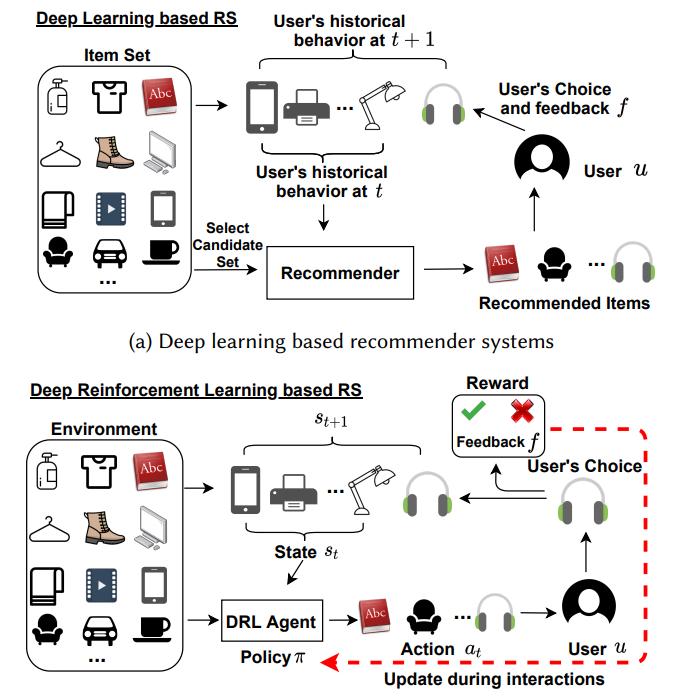
Given a set of users \(U\) = {𝑢, 𝑢1, 𝑢2, 𝑢3, …}, a set of items \(I\) = {𝑖, 𝑖1, 𝑖2, 𝑖3, …}, the system first recommends item 𝑖 to user 𝑢 and then gets feedback \(𝑓_i^u\). The system aims to incorporate the feedback to improve future recommendations and needs to determine an optimal policy \(\pi^*\) regarding which item to recommend to the user to achieve positive feedback. The MDP modelling of the problem treats the user as the environment and the system as the agent. The key components of the MDP in DRL-based RS include the following:
State \(S\): A state \(s_𝑡 ∈ S\) is determined by both users’ information and the recent 𝑙 items in which the user was interested before time 𝑡.
Action \(A\): An action \(𝑎_𝑡 ∈ A\) represents users’ dynamic preference at time 𝑡 as predicted by the agent. \(A\) represents the whole set of (potentially millions of) candidate items.
Transition Probability \(P\): The transition probability \(𝑝(𝑠_{𝑡+1}|𝑠_𝑡,𝑎_𝑡)\) is defined as the probability of state transition from \(𝑠_𝑡\) to \(𝑠_{𝑡+1}\) when action \(𝑎_𝑡\) is executed by the recommendation agent. In a recommender system, the transition probability refers to users’ behavior probability. \(P\) is only used in model-based methods.
Reward \(R\): Once the agent chooses a suitable action \(𝑎_𝑡\) based on the current state \(s_𝑡\) at time 𝑡, the user will receive the item recommended by the agent. Users’ feedback on the recommended item accounts for the reward \(𝑟(s_𝑡 , 𝑎_𝑡)\). The feedback is used to improve the policy 𝜋 learned by the recommendation agent.
Discount Factor 𝛾: The discount factor 𝛾 ∈ [0, 1] is used to balance between future and immediate rewards—the agent focuses only on the immediate reward when 𝛾 = 0 and takes into account all the (immediate and future) rewards otherwise.
The DRL-based recommendation problem can be defined by using MDP as follows. Given the historical MDP, i.e., \((S,A,P,R,\gamma)\), the goal is to find a set of recommendation policy ({𝜋} : S → A) that maximizes the cumulative reward during interaction with users.
Given an environment that contains all items I, when user 𝑢 ∈ U interacts with the system, an initial state 𝑠 is sampled from the environment which contains a list of candidate items and users’ historical data. The DRL agent needs to work out a recommendation policy 𝜋 based on the state 𝑠 and produces the corresponding recommended item list 𝑎. The user will provide feedback on the list which is normally represented as click or not click. The DRL agent will then utilize the feedback to improve the recommendation policy and move to the next interaction episode.
Simulation
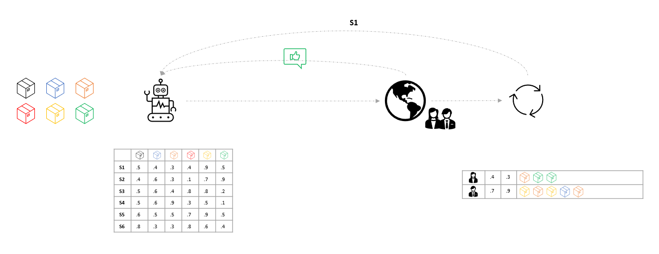
There are 4 components to build a recsys simulator.
User model - specifies which features are part of the user, and how they are generated (sampled from a distribution, or read from a dataset).
Item model - like the user model, this specifies which features describe an item.
User-choice model - generates user’s response to a particular item. This can be generated for example by sampling from a distribution, or by reading a matrix factorization of a user-interaction dataset. User-Choice models may also contain features like timestamps, user interactions, and so on.
User-transition model - determines how user features are affected after each user-item interaction. For instance, a user’s interest in a certain retail category may decrease after interacting with it. For instance, users might slowly get addicted to certain movie categories; this is simulated by slowly increasing user affinities (their embeddings obtained by the matrix factorization).
Challenges
Reinforcement learning is Agent-oriented learning, that is learning by interacting with an environment to achieve a goal. Which is learning by trial and error, with only delayed evaluative feedback (reward). It has been applied successfully to various problems, including robot control, power control, telecommunications, backgammon, checkers and Go. However RL does have some challenges: 1) We only have a reward signal as feedback, 2) Feedback is often delayed, 3) Time matters, sequential and non-stationary data, 4) Data received is affected by the agents previous interactions.
State-of-the-art recommender systems are notoriously hard to design and improve upon, due to their interactive and dynamic nature, since they involve a multi-step decision-making process, where a stream of interactions occurs between the user and the system. Leveraging reward signals from these interactions and creating a scalable and performant recommendation inference model is a key challenge. Traditionally, to make the problem tractable, the interactions are often viewed as independent, but in order to improve recommender systems further, the models will need to take into account the delayed effects of each recommendation and start reasoning/planning for longer-term user satisfaction.
Due to their interactive nature, recommender systems are also notoriously hard to evaluate. When evaluating their systems, practitioners often observe significant differences between a new algorithm’s offline and online results, and therefore tend to mostly rely on online methods, such as A/B testing. This is unfortunate, since online evaluation is not always possible and often expensive. Offline evaluation, on the other hand, provides a scalable way of comparing recommender systems and enables the participation of academic research in an industry-relevant problem.
In the past, recommender systems have been evaluated using proxy offline metrics coming from supervised methods, such as regression metrics (mean squared error, log likelihood), classification metrics (area under precision/recall curve) or ranking metrics (precision@k, normalized discounted cumulative gain). Recent research on recommender systems makes the link with counterfactual inference for offline A/B testing that reuses logged interaction data, and as well as the use of simulators that entirely avoid the use of potentially privacy-sensitive user data.
Moreover, a user’s interest (reward function) driving her behavior is typically unknown, yet it is critically important for the use of RL algorithms. In existing RL algorithms for recommendation systems, the reward functions are manually designed (e.g. ±1 for click/no-click) which may not reflect a user’s preference over different items.
Model-free RL typically requires lots of interactions with the environment in order to learn a good policy. This is impractical in the recommendation system setting. An online user will quickly abandon the service if the recommendation looks random and do not meet her interests.
There are a lot logged feedback from customers in recommender system, but subject to system biases caused by only observing feedback on recommendations selected by the previous versions of the recommender.
Also, It is difficult to apply reinforcement learning on recommender systems, because 1) it deals with large state and action spaces, 2) the set of items available to recommend is non-stationary and new items are brought into the system constantly, resulting in an ever-growing action space with new items having even sparser feedback, and 3) user preferences over these items are shifting all the time, resulting in continuously-evolving user states.
RL Tutorials
- Introduction to Gym toolkit
- Code-Driven Introduction to Reinforcement Learning
- CartPole using Cross-Entropy
- FrozenLake using Cross-Entropy
- FrozenLake using Value Iteration
- FrozenLake using Q-Learning
- CartPole using REINFORCE in PyTorch
- Cartpole in PyTorch
- Q-Learning on Lunar Lander and Frozen Lake
- REINFORCE
- Importance Sampling
- Kullback-Leibler Divergence
- MDP with Dynamic Programming in PyTorch
- REINFORCE in PyTorch
- MDP Basics with Inventory Control
- n-step algorithms and eligibility traces
- Q-Learning vs SARSA and Q-Learning extensions
RecSys Tutorials
- Multi-armed Bandit for Banner Ad
- Contextual Recommender with Vowpal Wabbit
- Top-K Off-Policy Correction for a REINFORCE Recommender System
- Neural Interactive Collaborative Filtering
- Batch-Constrained Deep Q-Learning
- Pydeep Recsys
- Recsim Catalyst
- Solving Multi-armed Bandit Problems
- Deep Reinforcement Learning in Large Discrete Action Spaces
- Off-Policy Learning in Two-stage Recommender Systems
- Comparing Simple Exploration Techniques: ε-Greedy, Annealing, and UCB
- Predicting rewards with the state-value and action-value function
- Real-Time Bidding in Advertising
- GAN User Model for RL-based Recommendation System
Citations
Off-policy Learning in Two-stage Recommender Systems. Jiaqi Ma, Zhe Zhao, Xinyang Yi, Ji Yang, Minmin Chen, Jiaxi Tang, Lichan Hong, Ed H. Chi. 2020. WWW. https://dl.acm.org/doi/pdf/10.1145/3366423.3380130
Reinforcement Learning based Recommender Systems: A Survey. M. Mehdi Afsar, Trafford Crump, Behrouz Far. 2021. arXiv. https://arxiv.org/abs/2101.06286
Optimized Recommender Systems with Deep Reinforcement Learning. Lucas Farris. 2021. arXiv. https://arxiv.org/abs/2110.03039v1
A Survey of Deep Reinforcement Learning in Recommender Systems: A Systematic Review and Future Directions. Xiaocong Chen, Lina Yao, Julian McAuley, Guanglin Zhou, Xianzhi Wang. 2021. arXiv. https://arxiv.org/abs/2109.03540
Interactive Search Based on Deep Reinforcement Learning. Yang Yu, Zhenhao Gu, Rong Tao, Jingtian Ge, Kenglun Chang. 2020. arXiv. https://arxiv.org/abs/2012.06052
Deep Reinforcement Learning With Python. Sudarshan. 2020. Oreilly. https://learning.oreilly.com/library/view/deep-reinforcement-learning/9781839210686/Text/Preface.xhtml
A Distributed Asynchronous Deep Reinforcement Learning Framework for Recommender Systems. Shi et. al.. 2020. RecSys. https://drive.google.com/file/d/1DULPZtXdUUnzNjwe3BQmD3sViOmYILCf/view
REVEAL 2020: Bandit and Reinforcement Learning from User Interactions. 2020. https://sites.google.com/view/reveal2020/
Proximal Policy Optimization Algorithms. John Schulman, Filip Wolski, Prafulla Dhariwal, Alec Radford, Oleg Klimov. 2017. arXiv. https://arxiv.org/abs/1707.06347
Offline Reinforcement Learning: Tutorial, Review, and Perspectives on Open Problems. Sergey Levine, Aviral Kumar, George Tucker, Justin Fu. 2020. arXiv. https://arxiv.org/abs/2005.01643
Reinforcement Learning for Recommender Systems: A Case Study on Youtube. Minmin Chen. 2019. RecSys. https://youtu.be/HEqQ2_1XRTs?list=PLN7ADELDRRhjH-LXON13wyKGN7nDOhcL1
Top-K Off-Policy Correction for a REINFORCE Recommender System. AISC. 2019. https://youtu.be/Ys3YY7sSmIA
Generative Adversarial User Model for Reinforcement Learning Based Recommendation System. Xinshi Chen, Shuang Li, Hui Li, Shaohua Jiang, Yuan Qi, Le Song. 2019. ICML. http://proceedings.mlr.press/v97/chen19f.html
Deep Reinforcement Learning based Recommendation with Explicit User-Item Interactions Modeling. Feng Liu, Ruiming Tang, Xutao Li, Weinan Zhang, Yunming Ye, Haokun Chen, Huifeng Guo, Yuzhou Zhang. 2018. arXiv. https://arxiv.org/abs/1810.12027
Deep Reinforcement Learning in Large Discrete Action Spaces. Gabriel Dulac-Arnold, Richard Evans, Hado van Hasselt, Peter Sunehag, Timothy Lillicrap, Jonathan Hunt, Timothy Mann, Theophane Weber, Thomas Degris, Ben Coppin. 2015. arXiv. https://arxiv.org/abs/1512.07679
Top-K Off-Policy Correction for a REINFORCE Recommender System. Minmin Chen, Alex Beutel, Paul Covington, Sagar Jain, Francois Belletti, Ed Chi. 2018. RecSys. https://arxiv.org/abs/1812.02353
Off-Policy Deep Reinforcement Learning without Exploration. Scott Fujimoto, David Meger, Doina Precup. 2018. arXiv. https://arxiv.org/abs/1812.02900
Value-aware Recommendation based on Reinforcement Profit Maximization. Changhua Pei , Xinru Yang , Qing Cui , Xiao Lin , Fei Sun , Peng Jiang , Wenwu Ou , Yongfeng Zhang Authors Info & Claims. 2019. WWW. https://dl.acm.org/doi/10.1145/3308558.3313404
Neural Interactive Collaborative Filtering. Lixin Zou , Long Xia , Yulong Gu , Xiangyu Zhao , Weidong Liu , Jimmy Xiangji Huang , Dawei Yin Authors Info & Claims. 2020. SIGIR. https://arxiv.org/abs/2007.02095
Reinforcement Learning - Industrial applications of intelligent agents. Phil Winder. 2020. Oreilly. https://learning.oreilly.com/library/view/reinforcement-learning/9781492072386/
Deep Reinforcement Learning Hands-On - Second Edition. Maxim Lapan. 2020. Oreilly. https://learning.oreilly.com/library/view/deep-reinforcement-learning/9781838826994/
Grokking Deep Reinforcement Learning. Miguel Morales. 2020. Oreilly. https://learning.oreilly.com/library/view/grokking-deep-reinforcement/9781617295454/
Mastering Reinforcement Learning with Python. Enes Bilgin. 2020. Oreilly. https://learning.oreilly.com/library/view/mastering-reinforcement-learning/9781838644147/
Deep Reinforcement Learning in Action. Alexander Zai, Bandon Brown. 2020. Manning. https://learning.oreilly.com/library/view/deep-reinforcement-learning/9781617295430/
Deep Reinforcement Learning with Python: With PyTorch, TensorFlow and OpenAI Gym. Nimish Sanghi. 2021. Oreilly. https://learning.oreilly.com/library/view/deep-reinforcement-learning/9781484268094/
Foundations of Deep Reinforcement Learning: Theory and Practice in Python. Laura Graesser, Wah Loon Keng. 2019. Oreilly. https://learning.oreilly.com/library/view/foundations-of-deep/9780135172490/
Deep Reinforcement Learning with Python - Second Edition. Sudharsan Ravichandiran. 2020. Oreilly. https://learning.oreilly.com/library/view/deep-reinforcement-learning/9781839210686/
The Reinforcement Learning Workshop. Alessandro Palmas, Emanuele Ghelfi, Dr. Alexandra Galina Petre, Mayur Kulkarni, Anand N.S., Quan Nguyen, Aritra Sen, Anthony So, Saikat Basak. 2020. Oreilly. https://learning.oreilly.com/library/view/the-reinforcement-learning/9781800200456/
PyTorch 1.x Reinforcement Learning Cookbook. Yuxi Liu. 2019. Oreilly. https://learning.oreilly.com/library/view/pytorch-1-x-reinforcement/9781838551964/
Reinforcement Learning Algorithms with Python. Andrea Lonza. 2019. Oreilly. https://learning.oreilly.com/library/view/reinforcement-learning-algorithms/9781789131116/
A Text-based Deep Reinforcement Learning Framework for Interactive Recommendation. Chaoyang Wang, Zhiqiang Guo, Jianjun Li, Peng Pan, Guohui Li. 2020. arXiv. https://arxiv.org/abs/2004.06651v4
DDPG: Continuous control with deep reinforcement learning. Timothy P. Lillicrap, Jonathan J. Hunt, Alexander Pritzel, Nicolas Heess, Tom Erez, Yuval Tassa, David Silver, Daan Wierstra. 2015. arXiv. https://arxiv.org/abs/1509.02971v6
Virtual-Taobao: Virtualizing Real-world Online Retail Environment for Reinforcement Learning. Jing-Cheng Shi, Yang Yu, Qing Da, Shi-Yong Chen, An-Xiang Zeng. 2018. arXiv. https://arxiv.org/abs/1805.10000
RecSim: A Configurable Simulation Platform for Recommender Systems. Eugene Ie, Chih-wei Hsu, Martin Mladenov, Vihan Jain, Sanmit Narvekar, Jing Wang, Rui Wu, Craig Boutilier. 2019. arXiv. https://arxiv.org/abs/1909.04847
RecoGym: A Reinforcement Learning Environment for the problem of Product Recommendation in Online Advertising. David Rohde, Stephen Bonner, Travis Dunlop, Flavian Vasile, Alexandros Karatzoglou. 2018. arXiv. https://arxiv.org/abs/1808.00720
Show Me the Whole World: Towards Entire Item Space Exploration for Interactive Personalized Recommendations. Yu Song, Jianxun Lian, Shuai Sun, Hong Huang, Yu Li, Hai Jin, Xing Xie. 2021. arXiv. https://arxiv.org/abs/2110.09905v1
Deep Reinforcement Learning for List-wise Recommendations. Xiangyu Zhao, Liang Zhang, Long Xia, Zhuoye Ding, Dawei Yin, Jiliang Tang. 2017. arXiv. https://arxiv.org/abs/1801.00209
Recommendations with Negative Feedback via Pairwise Deep Reinforcement Learning. Xiangyu Zhao, Liang Zhang, Zhuoye Ding, Long Xia, Jiliang Tang, Dawei Yin. 2018. arXiv. https://arxiv.org/abs/1802.06501
Stabilizing Reinforcement Learning in Dynamic Environment with Application to Online Recommendation. Chen et. al.. 2018. KDD. https://dl.acm.org/doi/epdf/10.1145/3219819.3220122
Reinforcement Knowledge Graph Reasoning for Explainable Recommendation. Yikun Xian, Zuohui Fu, S. Muthukrishnan, Gerard de Melo, Yongfeng Zhang. 2019. arXiv. https://arxiv.org/abs/1906.05237